Home

Context Navigation

Lagrangian particle model (LPM)

The embedded LPM allows for studying transport and dispersion processes within turbulent flows. In the following we will describe the general modeling of particles, including passive particles that do not show any feedback on the turbulent flow. In Sect. Lagrangian cloud model we will describe the use of Lagrangian particles as explicit cloud droplets.

Formulation of the LPM

Lagrangian particles can be released in prescribed source volumes at different points in time. The particles then obey

$\begin{align*} & \frac{\mathrm{d} x_{\mathrm{p}, i}}{\mathrm{d}t} = u_{\mathrm{p},i}(t) \end{align*}$

where x_p,i describes the particle location in x_i direction (i ∈ {1, 2, 3}) and u_p,i is the respective velocity component of the particle. Particle trajectories are calculated by means of the turbulent flow fields provided by PALM for each time step. The location of a certain particle at time t + Δ t_L is calculated by

$\begin{align*} & x_{\mathrm{p},i}(x_{\text{ps},i},t + \Delta t_\mathrm{L}) = x_{\mathrm{p},i}(x_{\text{ps},i},t) + \int \limits_t^{t + \Delta t_\mathrm{L}} u_{\mathrm{p},i}(\hat{t}) \mathrm{d}\hat{t}\,, \end{align*}$

where x_ps,i is the spatial coordinate of the particle source point and Δ t_L is the applied time step in the Lagrangian particle model. Note that the latter is not necessarily equal to the time step of the LES model. The integral in the Eq. above is evaluated using either a Runge-Kutta (2nd- or 3rd-order) or the (1st-order) Euler time-stepping scheme.

The velocity of a weightless particle that is transported passively by the flow is determined by

$\begin{align*} & u_{\mathrm{p},i} = u_i(x_{\mathrm{p},i})\;, \end{align*}$

and for non-passive particles (e.g., cloud droplets) by

$\begin{align*} & \frac{\mathrm{d}u_{\mathrm{p},i}}{\mathrm{d}t} = \frac{1}{\tau_\mathrm{p}} \left(u_i(x_{\mathrm{p},i}) - u_{\mathrm{p},i}\right) -\delta_{i3} \left(1 - \frac{\rho_0}{\rho_{\mathrm{l},0}} \right) g, \end{align*}$

considering Stoke's drag, gravity and buoyancy (on the right-hand side, from left to right). Note that this Eq. is solved analytically assuming all variables but u_p,i as constants for one time step. Here, u_i(x_p,i) is the velocity of air at the particles location gathered from the eight adjacent grid points of the LES by tri-linear interpolation (see Sect. particle code structure). Since Stoke's drag is only valid for radii ≤ 30 μm (e.g., Rogers and Yau, 1989), a nonlinear correction is applied to the Stokes's drag relaxation time scale:

$\begin{align*} & \tau_\mathrm{p}^{-1} = \frac{9\,\nu\,\rho_0}{2\,r^2\,\rho_{\mathrm{p},0}}\,\cdot\,\left(1 + 0.15 \cdot {Re}_\mathrm{p}^{0.687} \right). \end{align*}$

Here, r is the radius of the particle, ν = 1.461 x 10^-5 m² s the molecular viscosity of air, and ρ_p,0 the density of the particle. The particle Reynolds number is given by

$\begin{align*} & {Re}_\mathrm{p}=\frac{2\,r\,\left|\,u_i(x_{\mathrm{p},i}) - u_{\mathrm{p},i}\,\right|}{\nu}. \end{align*}$

Following Lamb (1978) and the concept of LES modeling, the Lagrangian velocity of a weightless particle can be split into a resolved-scale contribution u_p^res and an SGS contribution u_p^sgs:

$\begin{align*} u_{\mathrm{p},i} = u_{\mathrm{p},i}^{\text{res}} + u_{\mathrm{p},i}^{\text{sgs}}\,. \end{align*}$

u_p,i^res is determined by interpolation of the respective LES velocity components u_i to the position of the particle. The SGS part of the particle velocity at time t is given by

$\begin{align*} u_{\mathrm{p},i}^{\text{sgs}}(t) = u_{\mathrm{p},i}^{\text{sgs}}(t - \Delta t_\mathrm{L}) + \mathrm{d} u_{\mathrm{p},i}^{\text{sgs}}\,, \end{align*}$

where du_p,i^sgs describes the temporal change of the SGS particle velocity during a time step of the LPM based on Thomson (1987). Note that the SGS part of u_p,i in the second equation of this section is always computed using the (1st-order) Euler time-stepping scheme. Weil et al. (2004) developed a formulation of the Langevin equation under assumption of isotropic Gaussian turbulence in order to treat the SGS particle dispersion in terms of a stochastic differential equation. This equation reads as

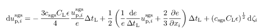
$\begin{align*} \mathrm{d}u_{\mathrm{p},i}^{\text{sgs}} = &-\frac{3 c_{\text{sgs}} C_\mathrm{L}\epsilon}{4}\frac{u_{\mathrm{p},i}^{\text{sgs}}}{e} \Delta t_\mathrm{L} + \frac{1}{2} \left(\frac{1}{e} \frac{\mathrm{d} e}{\Delta t_\mathrm{L}} u_{\mathrm{p},i}^{\text{sgs}} + \frac{2}{3}\frac{\partial e}{\partial x_i} \right) \Delta t_\mathrm{L} + \left(c_{\text{sgs}} C_\mathrm{L} \epsilon \right)^{\frac{1}{2}} \mathrm{d}\zeta_i\, \end{align*}$

and is used in PALM for the determination of the change in SGS particle velocities. Here, C_L = 3 is a universal constant (C_L = 4 ± 2, see Thomson (1987)). ζ is a vector composed of Gaussian-shaped random numbers, with each component neither spatially nor temporally correlated. The factor

$\begin{align*} c_\text{sgs} = \frac{\langle\,e\,\rangle}{\langle\,e_\text{res}\,\rangle + \langle\,e\,\rangle}\,,\quad 0 \leq c_\text{sgs} \leq 1\,, \end{align*}$

where e_res is the resolved-scale TKE as resolved by the numerical grid, assures that the temporal change of the modeled SGS particle velocities is, on average (horizontal mean), smaller than the change of the resolved-scale particle velocities (Weil et al., 2004). Values of e and ε are provided by the SGS model described in Sect. turbulence closure (see Eqs. for ∂e/∂t and for the dissipation rate ε,respectively). The first term on the right-hand side of the Eq. for du_p,i^sgs represents the influence of the SGS particle velocity from the previous time step (i.e., inertial "memory"). This effect is considered by the Lagrangian time scale after Weil et al. (2004):

$\begin{align*} \tau_\mathrm{L} = \frac{4}{3}\frac{e}{c_{\text{sgs}} C_\mathrm{L}\epsilon}\,, \end{align*}$

which describes the time span during which u_p^sgs(t - Δt_L) is correlated to u_p^sgs(t). The applied time step of the particle model hence must not be larger than τ_L. In PALM, the particle time step is set to be smaller than τ_L / 40. The second term on the right-hand side of the Eq. for du_p,i^sgs ensures that the assumption of well-mixed conditions by Thomson (1987) is fulfilled on the subgrid scales. This term can be considered as drift correction, which shall prevent an over-proportional accumulation of particles in regions of weak turbulence (#rodean1996 Rodean, 1996). The third term on the right-hand side is of stochastic nature and describes the SGS diffusion of particles by a Gaussian random process. For a detailed derivation and discussion of the Eq. for du_p,i^sgs see Thomson (1987), Rodean (1996) and Weil et al. (2004).

The required values of the resolved-scale particle velocity components, e, and ε are obtained from the respective LES fields using the eight adjacent grid points of the LES and tri-linear interpolation on the current particle location (see Sect. particle code structure). An exception is made in case of no-slip boundary conditions set for the resolved-scale horizontal wind components below the first vertical grid level above the surface. Here, the resolved-scale particle velocities are determined from MOST (see Sect. boundary conditions) in order to capture the logarithmic wind profile within the height interval of z₀ to z_MO. The available values of u_∗,

$$\overline{w^{\prime\prime}u^{\prime\prime}}_0$,$

and

$\overline{w^{\prime\prime}v^{\prime\prime}}_0$

are first bi-linearly interpolated to the horizontal location of the particle. In a second step the velocities are determined using the Eqs. for u_∗, ∂u/∂z and ∂v/∂z in Sect boundary conditions. Resolved-scale horizontal velocities of particles residing at height levels below z₀ are set to zero. The LPM allows to switch off the transport by the SGS velocities.

Boundary conditions and release of particles

Different boundary conditions can be used for particles. They can be either reflected or absorbed at the surface and top of the model. The lateral boundary conditions for particles can either be set to absorption or cyclic conditions.

The user can explicitly prescribe the release location and events as well as the maximum lifetime of each particle. Moreover, the embedded LPM provides an option for defining different groups of particles. For each group the horizontal and vertical extension of the particle source volumes as well as the spatial distance between the released particles can be prescribed individually for each source area. In this way it is possible to study the dispersion of particles from different source areas simultaneously.

Recent applications

The embedded LPM has been recently applied for the evaluation of footprint models over homogeneous and heterogeneous terrain (Steinfeld et al., 2008; Markkanen et al., 2009, 2010; Sühring et al., 2014). For example, Steinfeld et al. (2008) calculated vertical profiles of crosswind-integrated particle concentrations for continuous point sources and found good agreement with the convective tank experiments of Willis and Deardorff (1976), as well as with LES results presented by Weil et al. (2004). Moreover, Steinfeld et al. (2008) calculated footprints for turbulence measurements and showed the benefit of the embedded LPM for footprint prediction compared to Lagrangian dispersion models with fully parametrized turbulence. Noh et al. (2006) used the LPM to study the sedimentation of inertial particles in the OML. Moreover, the LPM has been used for visualizing urban canopy flows as well as dust-devil-like vortices (Raasch and Franke, 2011).

References

Rogers RR, Yau MK. 1989. A short course in cloud physics. Pergamon Press. New York.

Lamp RG. 1978. A numerical simulation of dispersion from an elevated point source in the convective planetary boundary layer. Atmos. Environ. 12: 1297–1304.

Thomson DJ. 1987. Criteria for the selection of stochastic models of particle trajectories in turbulent flows. J. Fluid Mech. 180: 529–556.

Weil JC, Sullivan PP, Moeng C-H. 2004. The use of large-eddy simulations in Lagrangian particle dispersion models. J. Atmos. Sci. 61: 2877–2887.

Rodean HC. 1996. Stochastic Lagrangian models of turbulent diffusion. Meteor. Mon. 26: 1–84. doi.

Steinfeld G, Raasch S, Markkanen T. 2008. Footprints in homogeneously and heterogeneously driven boundary layers derived from a Lagrangian stochastic particle model embedded into large-eddy simulation. Bound.-Lay. Meteorol. 129: 225–248.

Markkanen T, Steinfeld G, Kljun N, Raasch S, Foken T. 2009. Comparison of conventional Lagrangian stochastic footprint models against LES driven footprint estimates. Atmos. Chem. Phys. 9: 5575–5586. doi.

Markkanen T, Steinfeld G, Kljun N, Raasch S, Foken T. 2010. A numerical case study on footprint model performance under inhomogeneous flow conditions. Meteorol. Z. 19: 539–547.

Sühring M, Maronga B, Herbort F, Raasch S. 2014. On the effect of surface heat-flux heterogeneities on the mixed-layer top entrainment. Bound.-Lay. Meteorol. 151: 531–556.

Willis GE and Deardorff JW. 1976. A laboratory model of diffusion into the convective boundary layer. Q. J. Roy. Meteorol. Soc. 102: 427–445.

Noh Y, Kang IS, Herold M, Raasch S. 2006. Large-eddy simulation of particle settling in the ocean mixed layer. Phys. Fluids. 18: 085109. doi.

Raasch S, Franke T. 2011. Structure and formation of dust-devil-like vortices in the atmospheric boundary layer -- a high resolution numerical study. J. Geophys. Res. 116: D16120. doi.

Last modified 6 years ago Last modified on May 22, 2018 1:29:20 PM

Attachments (1)

Table5.png (38.6 KB) - added by schwenkel 6 years ago.

Download all attachments as: .zip

Download in other formats:

Plain Text