Home

Context Navigation

Subgrid-scale Model

One of the main challenges in LES modeling is the turbulence closure. The filtering process yields four SGS covariance terms (see the first five equations Sect. governing equations) that cannot be explicitly calculated. In PALM, three different subgrid-scale models are available to parameterize the SGS terms:

Selecting one of the available SGS models is done via the namelist parameter turbulence_closure.

Deardorff subgrid-scale model

In PALM, the default SGS model uses a 1.5-order closure according to Deardorff (1980). PALM applies the modified version of Moeng and Wyngaard (1988) and Saiki et al. (2000). The closure is based on the assumption that the energy transport by SGS eddies is proportional to the local gradients of the mean quantities and reads

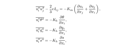
$\begin{align*} & \overline{u_i^{\prime\prime} u_j^{\prime\prime}} - \frac{2}{3} e \delta_{ij} = -K_\mathrm{m} \left(\frac{\partial u_{i}} {\partial x_{j}} + \frac{\partial u_j} {\partial x_{i}}\right),\,\\ & \overline{u^{\prime\prime}_{i}\theta^{\prime\prime}} = -K_\mathrm{h} \:\frac{\partial \theta} {\partial x_{i}},\,\\ & \overline{u^{\prime\prime}_{i}q^{\prime\prime}_\mathrm{v}} = -K_\mathrm{h} \:\frac{\partial q_\mathrm{v}} {\partial x_{i}},\,\\ & \overline{u^{\prime\prime}_{i}s^{\prime\prime}} = -K_\mathrm{h} \:\frac{\partial s}{\partial x_{i}},\, \end{align*}$

where K_m and K_h are the local SGS eddy diffusivities of momentum and heat, respectively. They are related to the SGS-TKE as follows

$\begin{align*} &K_\mathrm{m} = c_\mathrm{m}\;l\sqrt{e},\\ & K_\mathrm{h} = \left(1+\frac{2l}{\boldsymbol{\varDelta}}\right) K_\mathrm{m}. \end{align*}$

Here, c_m = 0.1 is a model constant and

$\begin{align*} & \boldsymbol{\varDelta} = \min\left( 1.8z, \left(\varDelta x \varDelta y \varDelta z \right)^{\frac{1}{3}} \right) \end{align*}$

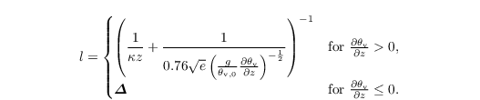
with Δx, Δy, Δz being the grid spacings in x, y and z direction, respectively. The SGS mixing length l depends on height z (distance from the wall when topography is used), grid spacing, and stratification and is calculated as

$\begin{align*} & l = \begin{cases} \min\left(\boldsymbol{\varDelta}, 0.76\sqrt{e}\left(\frac{g}{\theta_{\mathrm{v},0}} \frac{\partial{\theta_{\mathrm{v}}}}{\partial z}\right)^{-\frac{1}{2}} \right) &\text{for~} \frac{\partial{\theta_{\mathrm{v}}}}{\partial z} > 0, \\ \boldsymbol{\varDelta} &\text{for~} \frac{\partial{\theta_{\mathrm{v}}}}{\partial z} \leq 0. \end{cases} \end{align*}$

Moreover, the closure includes a prognostic equation for the SGS-TKE:

$\begin{align*} & \frac{\partial{e}}{\partial t} = - u_j\frac{\partial e}{\partial x_j} - \left(\overline{u_i^{\prime\prime} u_j^{\prime\prime}}\right)\frac{\partial u_i} {\partial x_j} + \frac{g}{\theta_{\mathrm{v},0}}\overline{u_3^{\prime\prime} {\theta_{\mathrm{v}}}^{\prime\prime}}-\frac{\partial}{\partial x_j} \left[\overline{u_j^{\prime\prime} \left(e + \frac{p^{\prime\prime}}{\rho_0}\right)}\right] - \epsilon. \end{align*}$

The pressure term in the equation above is parametrized as

$\begin{align*} &\left[\overline{u_j^{\prime\prime} \left(e + \frac{p^{\prime\prime}}{\rho_0}\right)}\right] = -2 K_\mathrm{m} \frac{\partial e}{\partial x_j} \end{align*}$

and ε is the SGS dissipation rate within a grid volume, given by

$\begin{align*} & \epsilon=\left(0.19 + 0.74\frac{l}{\boldsymbol{\varDelta}}\right)\frac{e^{\frac{3}{2}}}{l}. \end{align*}$

Since θ_v depends on θ, q_v, and q_l (see last equation Sect. governing equations), the vertical SGS buoyancy flux depends on the respective SGS fluxes (Stull, 1988, Chap. 4.4.5):

$\begin{align*} & \overline{w^{\prime\prime} {\theta_{\mathrm{v}}}^{\prime\prime}}=K_1\,\cdot\,\overline{w^{\prime\prime} {\theta}^{\prime\prime}} + K_2\,\cdot\,\overline{w^{\prime\prime} {q_\mathrm{v}}^{\prime\prime}}- \theta\,\cdot\,\overline{w^{\prime\prime} {q_\mathrm{l}}^{\prime\prime}}, \end{align*}$

with

$\begin{align*} & K_1 =1+\left(\frac{R_\mathrm{v}}{R_\mathrm{d}}-1\right) q_\mathrm{v} - q_\mathrm{l},\\ & K_2 =\left(\frac{R_\mathrm{v}}{R_\mathrm{d}}-1\right)\,\theta, \end{align*}$

and the vertical SGS flux of liquid water, calculated as

$\begin{align*} & \overline{w^{\prime\prime} {q_\mathrm{l}}^{\prime\prime}} = -K_\mathrm{h} \:\frac{\partial q_\mathrm{l}} {\partial z}. \end{align*}$

Note that this parametrization of the SGS buoyancy flux differs from that used with bulk cloud microphysics (see Sect. turbulence closure in cloud microphysics).

Modified Deardorff subgrid-scale model

A modificaiton of the Deardorff scheme described above is available that provides an improved mixing length calculation for locally stable stratification, particularly if used with fine grid spacings. Details about the deficiencies of the Deardorff scheme and the following modified version are given by Dai et al. (2020). In the following, we only describe the two modifications that are applied to the Deardorff scheme described above.

First, the mixing length is calculated as

$\begin{align*} & l = \begin{cases} \left(\dfrac{1}{\kappa z} +\dfrac{1}{0.76\sqrt{e}\left(\frac{g}{\theta_{\mathrm{v},0}} \frac{\partial{\theta_{\mathrm{v}}}}{\partial z}\right)^{-\frac{1}{2}} }\right)^{-1} &\text{for~} \frac{\partial{\theta_{\mathrm{v}}}}{\partial z} > 0, \\ \boldsymbol{\varDelta} &\text{for~} \frac{\partial{\theta_{\mathrm{v}}}}{\partial z} \leq 0. \end{cases} \end{align*}$

Seocnd, the eddy diffusivities are defined as

$\begin{align*} & K_h = \begin{cases} K_m & \text{for~} \frac{\partial{\theta_{\mathrm{v}}}}{\partial z} > 0, \\ 3 K_m & \text{for~} \frac{\partial{\theta_{\mathrm{v}}}}{\partial z} \leq 0. \end{cases} \end{align*}$

Note that this implementation has not been thoroughly tested yet. It is highly recommended to pay special attention and compare model results to runs with the default Deardorff model. Tests so far have revealed that the modified Deardorff scheme achieves grid convergence at relatively coarse grid spacings in simulations of the stable boundary layer (see Dai et al., 2020) and thus allows for using coarse grid spacings under such conditions (while still resolving the largest eddies). Note, however, that for fine grid spacings the eddy diffusivities are likely to be much higher than with the default Deardorff scheme, which can lead to significantly smaller time steps and thus higher computational costs.

Dynamic subgrid-scale model

The dynamic SGS model can be used as an alternative to the Moeng-Wyngaard version of the Deardorff model. In this case, K_m is calculated as

$\begin{align*} K_\mathrm{m} = c_*\;\Delta_\mathrm{max}\;\sqrt{e}, \end{align*}$

where Δ_max being the maximum of Δx, Δy, Δz. The calculation of c_* is based on an idea of Germano et al. (1991) to use a test filter, which is

$\begin{align*} \Delta_T = 2\Delta_\mathrm{max} \end{align*}$

in our case. The subgrid stress on the test filter scale is then

$\begin{align*} T_{ij} = \widehat{\overline{u_iu_j}} - \widehat{\overline{u}}_i\widehat{\overline{u}}_j \end{align*}$

(the hat denotes a filter operation on the test filter scale) which is also an unknown. The difference between subgrid stress on the test filter level and test filtered subgrid stress is described by the Germano identity

$\begin{align*} L_{ij} = T_{ij} - \widehat{\tau}_{ij} = \widehat{\overline{u}_i\overline{u}_j} - \widehat{\overline{u}}_i\widehat{\overline{u}}_j \end{align*}$

and can be calculated directly by application of the test filter on resolved quantities. c_* is then calculated via

$\begin{equation*} c_*=-\frac{L_{ij}^d\widehat{\overline{S}}^d_{ij}}{2\nu_t^T\widehat{\overline{S}}_{lk}^d\widehat{\overline{S}}_{kl}^d}, \end{equation*}$

where

$\begin{align*} \overline{S}_{ij} = \frac{1}{2}\left(\frac{\partial\overline{u_i}}{\partial x_j} + \frac{\partial\overline{u_j}}{\partial x_i} \right) \quad \mathrm{and} \quad \overline{S}^d_{ij} = \overline{S}_{ij} - \frac{1}{3}\overline{S}_{kk}\delta_{i,j} \end{align*}$

the strain tensor and the deviatoric strain tensor, repsectively, and ν_t the SGS viscosity. Unlike other dynamic models this formulation of c_* is not derived using model assumptions for the subgrid stress and the stress on the test filter level, but is based on proven turbulence properties (Heinz, 2008; Heinz and Gopalan, 2012). Furthermore, the stability of the simulation is ensured by using dynamic bounds that keep the values of c_* in the range

$\begin{equation*} |c_*| \leq \frac{23}{24\sqrt{3}}\frac{e^{1/2}}{\Delta|\overline{S}|}, \end{equation*}$

as was derived by Mokhtarpoor and Heinz (2017). This model does not need artificial clipping for stable runs and allows the occurence of backscatter (negative values of ν_t).

References

Dai, Y., Basu, S., Maronga, B., de Roode, SR. 2020. Addressing the Grid-size Sensititivty Issue in Large-eddy Simulations of Stable Boundary Layers. Boundary-layer Meteorol., submitted. http://arxiv.org/abs/2003.09463.

Deardorff JW. 1980. Stratocumulus-capped mixed layers derived from a three-dimensional model. Bound.-Lay. Meteorol. 18: 495–527.

Germano M., Piomelli U., Moin P., Cabot WH. 1991. A dynamic subgrid-scale eddy viscosity model. Physics of Fluids A 3: 1760–1765.

Heinz S. 2008. Realizability of dynamic subgrid-scale stress models via stochastic analysis. Monte Carlo Methods Appl. 14: 311-329.

Heinz S., Gopalan H. 2012. Realizable versus non-realizable dynamic subgrid-scale stress models. Physics of Fluids 24: 115105.

Moeng CH, Wyngaard JC. 1988. Spectral analysis of large-eddy simulations of the convective boundary layer. J. Atmos. Sci. 45: 3573–3587.

Mokhtarpoor R., Heinz S. 2017. Dynamic large eddy simulation: Stability via realizability. Physics of Fluids 29: 105104.

Saiki EM, Moeng CH, Sullivan PP. 2000. Large-eddy simulation of the stably stratified planetary boundary layer. Bound.-Lay. Meteorol. 95: 1–30.

Stull RB. 1988. An Introduction to Boundary Layer Meteorology. Kluwer Academic Publishers. Dordrecht. 666 pp.

Last modified 4 years ago Last modified on Feb 22, 2021 5:01:47 PM

Download in other formats:

Plain Text