
Direct Numerical Simulation
This chapter provides an example for a DNS validation run, where free convection over a heated plate was investigated. The reference for this simulation is case NsD from Mellado (2012). To save computational costs, the computationally cheaper case described in the appendix of Mellado (2012) is attached. In the following, some background knowledge is given, to explain the simulation setup.
Apart from RANS and LES simulations, PALM can also be used to perform Direct Numerical Simulations (DNSs). In contrast to the RANS mode, there is no need to adjust PALM's system of equations. DNSs can be performed by just using appropriate settings in the _p3d file. The following terms in the equation of motion differ from each other depending on the used mode (left from "≠" for DNS, right from "≠" for LES mode, more information can bee found at governing equations and subgrid-scale model):
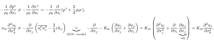
with π∗ = p∗ + 2/3 ρ0 e (the overbar indicating filtered quantities in LES mode is omitted ). Similar, also each convection–diffusion equation differs in one term (example for the potential temperature is shown):

Therefore, the governing equations implemented in the code are valid for DNS if a constant eddy diffusivity (Km) is used for the flow. In this way, no TKE is computed (e=0) and the not equal signs from the equation above change to equal signs. For DNS, the term eddy diffusivity is not valid anymore. Instead, we specify with km_constant the kinematic viscosity νm and molecular diffusivity νh for heat. In the medium air, these values are equal and have a magnitude of roughly 1.76e-5 if a Prandtl number of 1 is used.
The grid spacings Δ need to be comparable to the Kolmogorov length characterizing the smallest scales inside the turbulent region to ensure a DNS. With the general assumption that the Kolmogorov length is comparable to the diffusion length z0 characterizing the diffusive sublayer next to the wall, we can estimate Δ from, e.g. (see Mellado (2012))

with b0 being the surface buoyancy, which is given from the boundary condition. Due to the fine grid spacing, only several tens of seconds can be simulated. A simulation with an end time of 10s, 1024x1024x768 grid points, and grid spacings of 0.86e-3m needs about 1200 core hours on 512 CPUs already. Due to this short simulated time, the Coriolis force can be switched off.
The user code, which is also attached, can be used to provide similar initial conditions for the potential temperature/buoyancy profiles as described in Mellado (2012) and to calculate further quantities like the convection scale or the convective Rayleigh number.
References
- Mellado, J. P., 2012: Direct numerical simulation of free convection over a heated plate. J. Fluid Mech., 712, 418-450.
Attachments (2)
- ST_DNS_Validation_p3d (6.1 KB) - added by Giersch 6 years ago.
- user_module.f90 (40.7 KB) - added by Giersch 6 years ago.
Download all attachments as: .zip