Governing equations

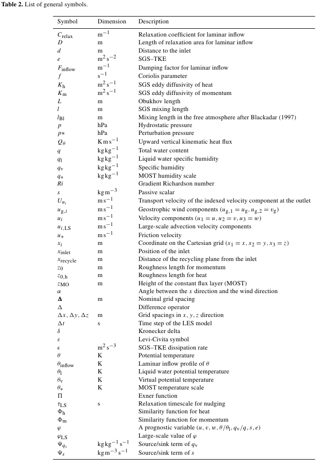
By default, PALM has seven prognostic quantities: the velocity components u, v, w on a Cartesian grid, the potential temperature θ, water vapor mixing ratio q_v, a passive scalar s, and the subgrid-scale turbulent kinetic energy (SGS-TKE) e. The separation of resolved scales and subgrid scales is implicitly achieved by averaging the governing equations over discrete Cartesian grid volumes as proposed by Schumann (1975). Moreover, it is possible to run PALM in a direct numerical simulation mode by switching off the prognostic equation for the SGS-TKE and setting a constant eddy diffusivity. For a list of all symbols and parameters, that we will introduce in this section, see the following Table 1 and 2.

The model is based on the non-hydrostatic, filtered, incompressible Navier-Stokes equations in Boussinesq-approximated form. In the following set of equations, angle brackets denote a horizontal domain average. A subscript 0 indicates a surface value. Note that the variables in the equations are implicitly filtered by the discretization (see above), but that the continuous form of the equations is used here for convenience. A double prime indicates SGS variables. The overbar indicating filtered quantities is omitted for readability, except for the SGS flux terms. The equations for the conservation of mass, energy and moisture, filtered over a grid volume on a Cartesian grid, then read as

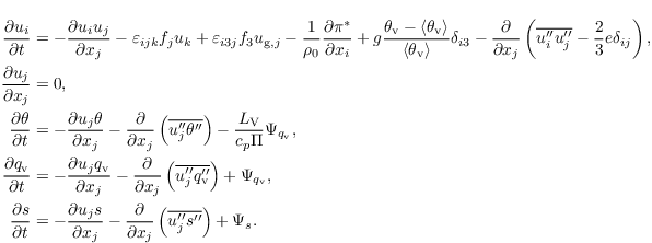
Here, i, j, k ∈ {1, 2, 3}. u_i are the velocity components (u₁ = u, u₂ = v, u₃ = w) with location x_i (x₁ = x, x₂ = y, x₃ = z), t is time, f_i = (-2 Ω cos(φ) sin(α), 2 Ω cos(φ) cos(α), 2 Ω sin(φ)) is the Coriolis parameter with Ω being the Earth's angular velocity, φ being the geographical latitude, and α being the (clockwise) rotation angle of the model domain. u_g,k are the geostrophic wind speed components, ρ₀ is the density of dry air, π^∗ = p^∗ + 2/3 ρ₀ e is the modified perturbation pressure with p^∗ being the perturbation pressure and the SGS-TKE

and g is the gravitational acceleration. The potential temperature is defined as

with the current absolute temperature T and the Exner function

with p being the hydrostatic air pressure, p₀ = 1000 hPa a reference pressure, R_d the specific gas constant for dry air, and c_p the specific heat of dry air at constant pressure. The virtual potential temperature is defined as

with the specific gas constant for water vapor R_v, and the liquid water mixing ratio q_l. For the computation of q_l, see the descriptions of the embedded cloud microphysical models in Sects. cloud microphysics and Lagrangian cloud model (LCM). Furthermore, L_V is the latent heat of vaporization, and Ψ_{q_v} and Ψ_s are source/sink terms of q_v and s, respectively.

References

• Schumann U. 1975. Subgrid scale model for finite difference simulations of turbulent flows in plane channels and annuli. J. Comput. Phys. 18: 376–404.