
Overview
TracNav
Core Parameters
Module Parameters
- Agent system
- Aerosol (Salsa)
- Biometeorology
- Bulk cloud physics
- Chemistry
- FASTv8
- Indoor climate
- Land surface
- Nesting
- Nesting (offline)
- Ocean
- Particles
- Plant canopy
- Radiation
- Spectra
- Surface output
- Synthetic turbulence
- Turbulent inflow
- Urban surface
- User-defined
- Virtual flights
- Virtual measurements
- Wind turbine
- Alphabetical list (outdated!)
This page is part of the Bulk Cloud Model (BCM) documentation.
It contains a listing of physical basics and the equations used.
For an overview of all BCM-related pages, see the Bulk Cloud Model main page.
PALM offers an embedded bulk cloud microphysics representation that takes into account cloud-microphysical processes for warm or mixed-phase clouds. Therefore, PALM solves the prognostic equations for the total water mixing ratio

instead of qv, and for a linear approximation of the liquid water potential temperature (e.g., Emanuel, 1994)

instead of θ as described in Sect. governing equations. Since q and θl are conserved quantities for wet adiabatic processes, condensation/evaporation is not considered for these variables.
PALM offers different schemes of (Kessler (1969), Seifert and Beheng (2001,2006), Morrison et al. (2007)) for the treatment of liquid phase microphysics. Depending of the choice of the microphysical scheme the different prognostic quantities are use and different microphysical processes are considered. In the following the schemes and their underlying processes are introduced.
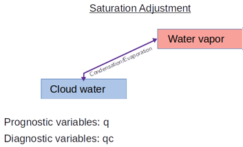
Saturation Adjustment Actually, the saturation adjustment scheme does not represent s particular microphysics scheme. It just converts the excess supersaturation into liquid water by neglecting all other microphysical processes. |
|

Kessler The Kessler (1969) scheme provides a computational inexpensive way for the bulk microphysics. However, it only converts supersaturation into liquid water and considering autoconversion after a parameterization of Kessler (1969). |
|

Seifert and Beheng A more detailed parameterization is given by following the two-moment scheme of Seifert and Beheng (2001,2006), which is based on the separation of the droplet spectrum into droplets with radii < 40 μm (cloud droplets) and droplets with radii ≥ 40 μm (rain droplets). Here, the model predicts the first two moments of these partial droplet spectra, namely cloud and rain droplet number concentration (Nc and Nr, respectively) as well as cloud and rain water mixing ratio (qc and qr, respectively). Consequently, ql is the sum of both qc and qr. The moments' corresponding microphysical tendencies are derived by assuming the partial droplet spectra to follow a gamma distribution that can be described by the predicted quantities and empirical relationships for the distribution's slope and shape parameters. For a detailed derivation of these terms, see Seifert and Beheng (2001,2006). We employ the computational efficient implementation of this scheme as used in the UCLA-LES (Savic-Jovcic and Stevens, 2008) and DALES (Heus et al., 2010) models. We thus solve only two additional prognostic equations for Nr and qr:  with the sink/source terms ΨNr and Ψqr, and the SGS fluxes  with Nc and qc being a fixed parameter and a diagnostic quantity, respectively. |
|

Morrison The Morrison et al. (2007) microphysics scheme can be understood as an extension of the scheme of Seifert and Beheng (2001,2006), where Nc and qc are prognostic quantities as well.  with the sink/source terms ΨNc and Ψqc, and the SGS fluxes  Moreover, using the Morrison et al. (2007) scheme includes an explicit calculation of diffusional growth and an activation parameterization. |
|

Morrison no rain Instead of using the Morrison scheme as an extension of the Seifert and Beheng (2001,2006) scheme, the extension are used as a stand-alone scheme. Therefore, rain processes are neglected but explicit consideration of diffusional growth and activation with prognostic quantities of Nc and qc. This scheme is computational inexpensive and appropriate for conditions where the production of rain can be neglected (i.e. fog). |
|

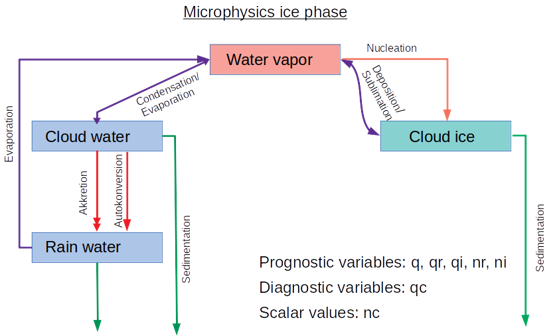
Mixed phase microphysics Note, that at the mixed phase bulk microphysics is still under development but can already applied. However, instead of prescribing it as an own scheme (as the others) it must be turned on as with ... and is implemented as an extension of the schemes of Seifert and Beheng (2006) and Morrison et al. (2007). At this state only processes for ice crystal are included involving two further prognostic quantities: ice crystal number Ni and ice crystal mixing ratio qi. Thus additional prognostic equations for Ni and qi are solved:  with the sink/source terms ΨNi and Ψqi, and the SGS fluxes  |
|

In the next subsections we will describe the diagnostic/prognostic determination (in dependence of the chosen scheme) of qc. From Sect. autoconversion on, the microphysical processes considered in the sink/source terms of θl, q, Nr and qr and Ni and qi, as well as Nc and qc for the Morrison et al. (2007) scheme.
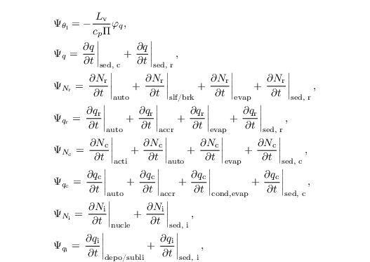
are used in the formulations of Seifert and Beheng (2006) unless explicitly specified. Section turbulence closure gives an overview of the necessary changes for the turbulence closure (cf. Sect. turbulence closure) using q and θl instead of qv and θ, respectively.

Activation of cloud droplets
The use of the Morrison et al. (2007) scheme enables a prognostic equation for the cloud droplet number concentration. Here, it is assumed that cloud droplets are activated in dependence of the current supersaturation. This basic method is called Twomey activation scheme with the general form of

where NCCN is the number of activated aerosols, N0 is the number concentration of dry aerosol, S is the supersaturation and k is power index between 0 and 1. In PALM the supersaturation is calculated explicitly by their thermodynamic fields of potential temperature and water vapor mixing ratio. However, curvature and solution effects can be considered with an analytical extension of the Twomey type activation scheme of Khvorostyanov and Curry (2006). By doing so, the number of activated aerosol is calculated by
![\begin{align*}
& N_\mathrm{CCN}=\frac{N_\mathrm{0}}{2} [1-\text{erf}(u)];\hspace{1.5cm} u = \frac{\ln(S_\mathrm{0}/S)}{\sqrt{2} \ln \sigma_\mathrm{s}}
\end{align*}](/trac/tracmath/951c2d3d1ebb5a53ef8b51f85d5df060b32d4c00.png)
where erf is the Gaussian error function, and

Here A is the Kelivn parameter and b and β depend on the chemical composition and physical properties of the dry aerosol. Since aerosol is not predicted in this scheme, the number of aerosols previously activated is assumed to be equal to the number of droplets Nc. Therefore, the actual activation rate is given by

Diffusional growth of cloud water
By the usage of Seifert and Beheng (2001,2006) scheme the diagnostic estimation of qc is based on the assumption that water supersaturations are immediately removed by the diffusional growth of cloud droplets only. This can be justified since the bulk surface area of cloud droplets exceeds that of rain drops considerably (Stevens and Seifert, 2008). Following this saturation adjustment approach, qc is obtained by

where qs is the saturation mixing ratio. Because qs is a function of T (not predicted), qs is computed from the liquid water temperature Tl = Π θl in a first step:

using an empirical relationship for the saturation water vapor pressure pv,s (Bougeault, 1981):

qs(T) is subsequently calculated from a 1st-order Taylor series expansion of qs at Tl (Sommeria and Deardorff, 1977):

with

In contrast to that an explicit approach for the diffusional growth is applied in case of Morrison et al. (2007). The condensation rate is calculated following Khairoutdinov and Kogan (2000) and given by

where S is the supersaturation, Rc the integral radius and G(T,p) a function of temperature and pressure considering heat conductivity and diffusion. Using this explicit approach the used timestep must fulfill a new criterion, since it is assumed that the supersaturation is constant during one timestep. The typical diffusion timescale is given by Arnason and Brown (1971) with

with

However, in PALM this criterion is not explicitly checked. Too ensure that unrealistic condensation or evaporation rates are avoided this scheme is limited to the value of the saturation-adjustment scheme.
Autoconversion
In the following Sects. Autoconversion - Self-collection and breakup we describe collision and coalescence processes by applying the stochastic collection equation (e.g., Pruppacher and Klett, 1997, Chap. 15.3) in the framework of the described two-moment scheme. As two species (cloud and rain droplets, hereafter also denoted as c and r, respectively) are considered only, there are three possible interactions affecting the rain quantities: autoconversion, accretion, and selfcollection. Autoconversion summarizes all merging of cloud droplets resulting in rain drops (c + c → r). Accretion describes the growth of rain drops by the collection of cloud droplets (r + c → r). Selfcollection denotes the merging of rain drops (r + r → r).
The local temporal change of qr due to autoconversion is
![\begin{align*}
& \left.\frac{\partial q_\mathrm{r}}{\partial t}
\right|_{\text{auto}}=\frac{K_{\text{auto}}}{20\,m_{\text{sep}}}\frac{(\mu_\mathrm{c} +2)
(\mu_\mathrm{c} +4)}{(\mu_\mathrm{c} + 1)^2} q_\mathrm{c}^2
m_\mathrm{c}^2 \cdot \left[1+
\frac{\Phi_{\text{auto}}(\tau_\mathrm{c})}{(1-\tau_\mathrm{c})^2}\right]
\rho_0.
\end{align*}](/trac/tracmath/ef58d69eeb8e613e0b970b3700a2e0ec2f7754c5.png)
Assuming that all new rain drops have a radius of 40 μm corresponding to the separation mass msep = 2.6 x 10⁻¹⁰ kg, the local temporal change of Nr is

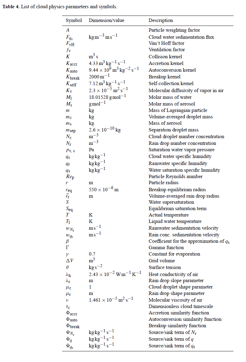
Here, Kauto = 9.44 x 10⁹ m3 kg-2 s-1 is the autoconversion kernel, μc = 1 is the shape parameter of the cloud droplet gamma distribution and mc = ρ qc / Nc is the mean mass of cloud droplets. τc = 1 - qc / (qc + qr) is a dimensionless timescale steering the autoconversion similarity function

The increase of the autoconversion rate due to turbulence can be considered optionally by an increased autoconversion kernel depending on the local kinetic energy dissipation rate after Seifert et al. (2010).
Accretion
The increase of qr by accretion is given by:

with the accretion kernel Kaccr = 4.33 m3 kg-1 s-1 and the similarity function

Turbulence effects on the accretion rate can be considered after using the kernel after Seifert et al. (2010).
Self-collection and breakup
Selfcollection and breakup describe merging and splitting of rain drops, respectively, which affect the rain water drop number concentration only. Their combined impact is parametrized as

with the breakup function

depending on the volume averaged rain drop radius

the equilibrium radius req = 550 x 10-6 m and the breakup kernel Kbreak = 2000 m-1. The local temporal change of Nr due to selfcollection is

with the selfcollection kernel Kself = 7.12 m3 kg-1 s-1.
Evaporation of rainwater
The evaporation of rain drops in subsaturated air (relative water supersaturation S < 0) is parametrized following Seifert (2008):

where
![\begin{align*}
& G = \left[\frac{R_\mathrm{v}T}{K_\mathrm{v}p_\text{v, s}(T)} +
\left(\frac{L_\mathrm{V}}{R_\mathrm{v} T}-1\right)
\frac{L_\mathrm{V}}{\lambda_\mathrm{h}\,T}\right]^{-1},
\end{align*}](/trac/tracmath/4199d403125ca15056ce5c71e4c6d5550d9a4887.png)
with Kv = 2.3 x 10⁻⁵ m2 s-1 being the molecular diffusivity water vapor in air and λh = 2.43 x 10⁻² W m-1 K-1 being the heat conductivity of air. Here, Nr λrμr+1 / Γ(μr+1) denotes the intercept parameter of the rain drop gamma distribution with Γ being the gamma-function. Following Stevens and Seifert (2008), the slope parameter reads as

with μr being the shape parameter, given by

In order to account for the increased evaporation of falling rain drops, the so-called ventilation effect, a ventilation factor fv is calculated optionally by a series expansion considering the rain drop size distribution (Seifert, 2008, Appendix).
The complete evaporation of rain drops (i.e., their evaporation to a size smaller than the separation radius of 40 µm) is parametrized as

with γ = 0.7 (see also Heus et al., 2010).
Sedimentation of cloudwater
As shown by Ackerman et al. (2009), the sedimentation of cloud water has to be taken in account for the simulation of stratocumulus clouds. They suggest the cloud water sedimentation flux to be calculated as

based on a Stokes drag approximation of the terminal velocities of log-normal distributed cloud droplets. Here, k = 1.2 x 10⁸ m-1 s-1 is a parameter and σg = 1.3 the geometric SD of the cloud droplet size distribution (Geoffroy et al., 2010). The tendency of q results from the sedimentation flux divergences and reads as

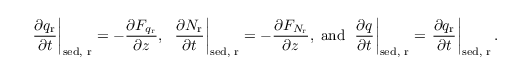
Sedimentation of rainwater
The sedimentation of rain water is implemented following Stevens and Seifert (2008). The sedimentation velocities are based on an empirical relation for the terminal fall velocity after Rogers et al. (1993). They are given by

and

The resulting sedimentation fluxes FNr and Fqr are calculated using a semi-Lagrangian scheme and a slope limiter (see Stevens and Seifert, 2008, their Appendix A). The resulting tendencies read as
Turbulence closure
Using bulk cloud microphysics, PALM predicts liquid water temperature θl and total water mixing ratio q instead of θ and qv. Consequently, some terms in the Eq. for

of Sect. turbulence closure are unknown. We thus follow Cuijpers and Duynkerke (1993) and calculate the SGS buoyancy flux from the known SGS fluxes

and

In unsaturated air (qc = 0) the Eq. for

of Sect. turbulence closure is then replaced by

with

and in saturated air (qc > 0) by

Attachments (8)
- Table4.png (114.2 KB) - added by westbrink 6 years ago.
- saturation-adjustment.png (25.8 KB) - added by schwenkel 5 years ago.
- saturation-adjustment.2.png (23.2 KB) - added by schwenkel 5 years ago.
- seifert_and_beheng.png (45.1 KB) - added by schwenkel 5 years ago.
- morrison.png (36.6 KB) - added by schwenkel 5 years ago.
- morrison_no_rain.png (28.6 KB) - added by schwenkel 5 years ago.
- kessler.png (30.4 KB) - added by schwenkel 5 years ago.
- mixed_phase.png (56.5 KB) - added by schwenkel 5 years ago.
Download all attachments as: .zip