
| Version 2 (modified by Giersch, 9 years ago) (diff) |
|---|
This site is currently under construction!
Lagrangian particle model (LPM)
The embedded LPM allows for studying transport and dispersion processes within turbulent flows. In the following we will describe the general modeling of particles, including passive particles that do not show any feedback on the turbulent flow. In Sect. Lagrangian cloud model we will describe the use of Lagrangian particles as explicit cloud droplets.
Formulation of the LPM
Lagrangian particles can be released in prescribed source volumes at different points in time. The particles then obey

where xp,i describes the particle location in xi direction (i ∈ {1, 2, 3}) and up,i is the respective velocity component of the particle. Particle trajectories are calculated by means of the turbulent flow fields provided by PALM for each time step. The location of a certain particle at time t + Δ tL is calculated by
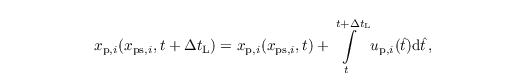
where xps,i is the spatial coordinate of the particle source point and Δ tL is the applied time step in the Lagrangian particle model. Note that the latter is not necessarily equal to the time step of the LES model. The integral in the Eq. above is evaluated using either a Runge-Kutta (2nd- or 3rd-order) or the (1st-order) Euler time-stepping scheme.
The velocity of a weightless particle that is transported passively by the flow is determined by

and for non-passive particles (e.g., cloud droplets) by
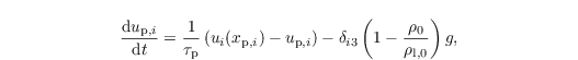
considering Stoke's drag, gravity and buoyancy (on the right-hand side, from left to right). Note that this Eq. is solved analytically assuming all variables but up,i as constants for one time step. Here, ui(xp,i) is the velocity of air at the particles location gathered from the eight adjacent grid points of the LES by tri-linear interpolation (see Sect. particle code structure).
Boundary conditions and release of particles
Recent applications
Attachments (1)
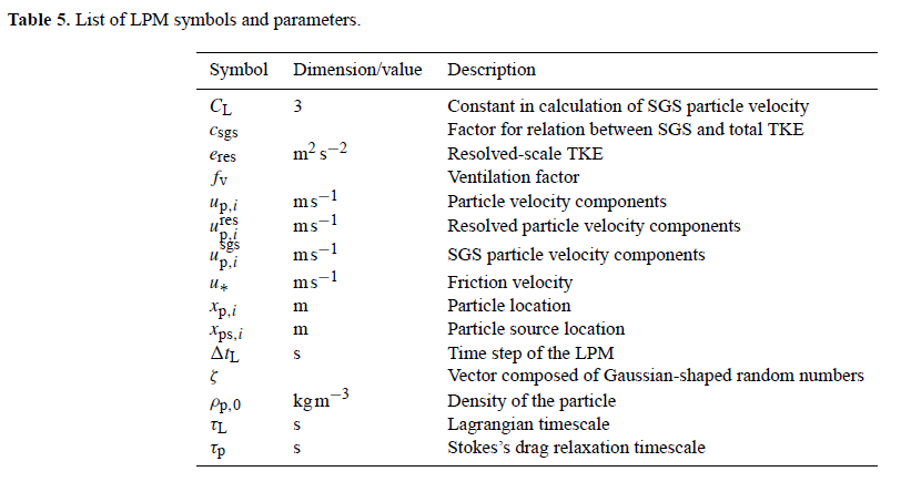
- Table5.png (38.6 KB) - added by schwenkel 7 years ago.
Download all attachments as: .zip