
Discretization
Spatial discretization
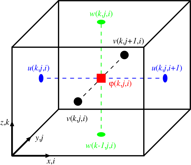
The model domain in PALM is discretized in space using finite differences and equidistant horizontal grid spacings (Δx, Δy). The grid can be stretched in the vertical direction well above the ABL to save computational time in the free atmosphere. The Arakawa staggered C-grid (Harlow and Welch, 1965; Arakawa and Lamb, 1977) is used, where scalar quantities are defined at the center of each grid volume, whereas velocity components are shifted by half a grid width in their respective direction so that they are defined at the edges of the grid volumes (see Fig. 1).
The bottom boundary of the model domain is indicated by the first w-component (w(k=0)) whereas the top boundary is indicated by w(k=nz). The first grid point for scalars and u,v is always defined at the same height as w(k=0) (0m). At the top boundary, the last scalar grid point (nz+1) is dz/2 above w(k=nz). However, if you like to have exactly symmetric vertical boundaries (i.e. the same grid structure / grid spacing at bottom and top), shifting the uppermost grid point for scalars and u,v to the height of w(k=nz) is required. In addition, a symmetric behavior between bottom and top boundary requires additional changes in the reduction of the order of the advection scheme close to the boundaries. These changes and the adjustments to a strictly symmetric grid structure can be switched on via parameter setting topography = 'closed_channel'.
Note: Due to same array sizes of u, v, and w the uppermost grid point of the model domain is w(k=nz+1). This point doesn't play a role for solving the model equations.

Figure 1: The Arakawa staggered C-grid. The indices i, j, k refer to grid points in x, y and z direction, respectively. Scalar quantities φ are defined at the center of the grid volume, whereas velocities are defined at the edges of the grid volumes.
It is thus possible to calculate the derivatives of the velocity components at the center of the volumes (same location as the scalars). By the same token, derivatives of scalar quantities can be calculated at the edges of the volumes. In this way it is possible to calculate derivatives over only one grid length and the effective spatial model resolution can be increased by a factor of two in comparison to non-staggered grids. By default, the advection terms in the first five equations in Sect. governing equations are discretized using an upwind-biased 5th-order differencing scheme in combination with a 3rd-order Runge–Kutta time-stepping scheme after Williamson (1980). Wicker and Skamarock(2002) compared different time- and advection differencing schemes and found that this combination give the best results regarding accuracy and algorithmic simplicity. However, the 5th-order differencing scheme is known to be overly dissipative. It is thus also possible to use a 2nd-order scheme after Piacsek and Williams(1970). The latter scheme is non-dissipative, but it suffers from immense numerical dispersion. Time discretization can also be achieved using 2nd-order Runge–Kutta or 1st-order Euler schemes. For more information about the advection and time differencing schemes see Higher order advection scheme and time integration.
Higher order advection scheme
Based on a flux formulation of the advection term

the one dimensional advection equation can be written in the following semidiscrete form:

where

denotes the fluxes staggered half a grid length related to the advected quantity.
Wicker and Skamarock (2002) discretized the 6th and 5th order fluxes as follows:
![\begin{align*}
F_{i-\frac{1}{2}}^{6} = \frac{u_{i-\frac{1}{2}}}{60} \left[ 37(\psi_{i}+\psi_{i-1}) - 8(\psi_{i+1} + \psi_{i-2}) +(\psi_{i+2} + \psi_{i-3}) \right] ,
\end{align*}](/trac/tracmath/ea3d33d8e13c34a7cae7976bf9a7068b4d0ddee9.png)
![\begin{align*}
F_{i-\frac{1}{2}}^{5} = F_{i-\frac{1}{2}}^{6} - \dfrac{|u_{i-\frac{1}{2}}|}{60} \left[10(\psi_{i}-\psi_{i-1}) -5(\psi_{i+1} - \psi_{i-2})+(\psi_{i+2} - \psi_{i-3}) \right] .
\end{align*}](/trac/tracmath/444d2f6a945150702636d75fd29e1dedcbf696e1.png)
The 5th order upwind discretization (WS5) consists of a centered non dissipative 6th (WS6) order flux and an artificially added numerical dissipation term. This term is necessary to stabilize the numerical solution, because higher order centered fluxes exhibits worse stability properties. The absolute value of the advective velocity component in the dissipation term removes a sign-dependent effect of the velocity and assures a dissipative effect also for u < 0.
Numerical properties
A semidiscrete fourier transformation for the spatial derivatives maps the one dimensional advection equation in fourier space as follows (Baldauf, 2008):

where

denotes the fourier transformed of ψ. The Courant number

characterizes stability properties and i is the imaginary unit. κeff is the effective wavenumber of a mode in fourier space and characterizes the modified wavenumber through the discretization. The real part of the effective wavenumber describes the dispersion error, the imaginary part the dissipation error.

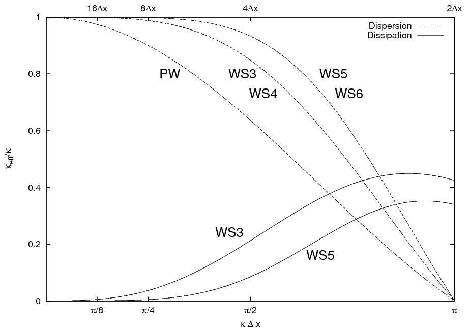
Figure 2: The dispersion and dissipation error as a function of the dimensionless wavenumber κ Δx for WS3 (3rd order scheme), WS4 (4th order scheme), WS5, WS6 and the 2nd order scheme of Piacsek and Williams (1970) (PW).
Fig. 2 shows that the dispersion error of the upwind schemes and the dispersion error of the next higher, even ordered scheme are identical. Generally the dispersion error decreases with increasing order of the discretization. However, no of the depicted schemes is able to adequately resolve structures with wavelengths near 2-Δx (generally no scheme based on finite differences is capable to do this). The centered, even ordered schemes hold no dissipation errors. With increasing order the numerical dissipation is more local. So the maximum wavelength affected by the dissipation term is round about 8-Δx with WS5, whereas wavelength of 16-Δx are still affected with WS3. Accordingly to the maximum of the amplification factor at κ Δx = 1.69 (these waves become unstable at first) in conjunction with the used Runge-Kutta method (Baldauf, 2008), the 5th order dissipation is sufficient to avoid instabilities. The maximum stable Courant-number is Cr = 1.4 (Baldauf, 2008).
Note: A stable numerical solution can only be guaranteed with the 3 rd order Runge-Kutta method.
Boundaries
Due to the seven-point stencil of WS5, three ghost layers are required on each lateral boundary of the processor subdomains, in order to avoid local data dependencies. Therefore, the exchange of ghost layers is adapted to a dynamic number of ghost layers, depending on the applied advection scheme. Near the bottom and top boundaries, as well as near lateral non-cyclic boundaries and near topography walls, the order of the discretization is successively degraded from fifth order to a third-order scheme and further to a first-order scheme. The degradation is controlled by three-dimensional bit flags, where several bits mark the order of the advection scheme in the x-, y-, and z-direction. Technically, in case of WS-scheme advective fluxes are calculated for the first-, third-, and fifth-order descretization, while the respective bit controls which discretization is finally used. In the following, the respective flags are listed:
| Array | Bit | Meaning |
|---|---|---|
adv_flags_s | 0 | scalar advection in the x-direction: first order |
adv_flags_s | 1 | scalar advection in the x-direction: third order |
adv_flags_s | 2 | scalar advection in the x-direction: fifth order |
adv_flags_s | 3 | scalar advection in the y-direction: first order |
adv_flags_s | 4 | scalar advection in the y-direction: third order |
adv_flags_s | 5 | scalar advection in the y-direction: fifth order |
adv_flags_s | 6 | scalar advection in the z-direction: first order |
adv_flags_s | 7 | scalar advection in the z-direction: third order |
adv_flags_s | 8 | scalar advection in the z-direction: fifth order |
adv_flags_s | 0 | u advection in the x-direction: first order |
adv_flags_m | 1 | u advection in the x-direction: third order |
adv_flags_m | 2 | u advection in the x-direction: fifth order |
adv_flags_m | 3 | u advection in the y-direction: first order |
adv_flags_m | 4 | u advection in the y-direction: third order |
adv_flags_m | 5 | u advection in the y-direction: fifth order |
adv_flags_m | 6 | u advection in the z-direction: first order |
adv_flags_m | 7 | u advection in the z-direction: third order |
adv_flags_m | 8 | u advection in the z-direction: fifth order |
adv_flags_m | 9 | v advection in the x-direction: first order |
adv_flags_m | 10 | v advection in the x-direction: third order |
adv_flags_m | 11 | v advection in the x-direction: fifth order |
adv_flags_m | 12 | v advection in the y-direction: first order |
adv_flags_m | 13 | v advection in the y-direction: third order |
adv_flags_m | 14 | v advection in the y-direction: fifth order |
adv_flags_m | 15 | v advection in the z-direction: first order |
adv_flags_m | 16 | v advection in the z-direction: third order |
adv_flags_m | 17 | v advection in the z-direction: fifth order |
adv_flags_m | 18 | w advection in the x-direction: first order |
adv_flags_m | 19 | w advection in the x-direction: third order |
adv_flags_m | 20 | w advection in the x-direction: fifth order |
adv_flags_m | 21 | w advection in the y-direction: first order |
adv_flags_m | 22 | w advection in the y-direction: third order |
adv_flags_m | 23 | w advection in the y-direction: fifth order |
adv_flags_m | 24 | w advection in the z-direction: first order |
adv_flags_m | 25 | w advection in the z-direction: third order |
adv_flags_m | 26 | w advection in the z-direction: fifth order |
Statistical evaluation of turbulent fluxes
In case of lower order advection scheme, e.g. the Piascek-Williams scheme, the turbulent flux of a quantity s is calculated by the so-called spatial eddy covariance method,

where w is the vertical velocity. The overbar denotes the spatial mean, while the angle brackets denote a temporal mean.
However, in case of higher order advection scheme, the statistical evaluation of a turbulent flux is not consistent with the way how the flux is treated in the model by the advection scheme, due to the different spatial stencil. As a consequence, in case of higher-order advection scheme, some unphysical kinks occur in the turbulent flux profiles if spatial eddy covariance is used, especially near the ground where the turbulent transport is poorly resolved. This is also known as statistical evaluation problem.
In order to circumvent this problem in case of higher-order advection scheme, turbulent fluxes are calculated the same way as they are treated by the advection scheme, i.e. they are calculated directly in the advection routines and are reused later for statistical output.
This case, the statistical output reads as:

where the second term removes the mean part of the transport.
In case of higher-order advection, turbulent fluxes are evaluated on each Runge-Kutta substep and weighted with the respective Runge-Kutta coefficients to remove dependencies of the Runge-Kutta substeps.
Temporal discretization
For the discretization in time a 3rd order low-storage Runge-Kutta scheme with 3 stages is used recommended by Williamson (1980). Generally an N-stage Runge-Kutta scheme discretizes an ordinary differential equation of the form

as follows (Baldauf, 2008):
![\begin{align*}
\psi^{(0)} &= \psi^{n}, \\
k^{i} &= f(t^{n} + \Delta t\,\alpha_{i},\,\psi^{i-1}), \\
\psi^{i} &= \psi^{n} + \Delta t\,\sum^{i}_{j=1}\,\beta_{i+1,j}\,k^{j}, \quad \textnormal{mit} \quad i \in [1,2,...,N] \\
\psi^{n+1} &= \psi^{N}.
\end{align*}](/trac/tracmath/6638ebaeebd31d91fa4c35066111efb0834a67e6.png)
The coefficients can be written in a so-called Butcher-Tableau:
| α1 | β1,1 | 0 | ... | ||
| α2 | β2,1 | β2,2 | 0 | ... | |
| ... | ... | ||||
| αN | βN,1 | βN,2 | ... | βN,N-1 | 0 |
| βN+1,1 | βN+1,2 | ... | βN+1,N-1 | βN+1,N |
The appendant coefficients for the applied Runge-Kutta scheme reads:
| 0 | 0 | 0 | 0 |
| 1/3 | 1/3 | 0 | 0 |
| 3/4 | -3/16 | 15/16 | 0 |
| 1/6 | 3/10 | 8/15 |
To save storage it is advantageous to compute ψN from the intermediate solutions ψ1 and ψ2 and combine the local tendencies in one array after the second substep (therefore low-storage scheme) as follows:
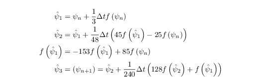
For reasons of clarity the time integration for several schemes (further schemes are: Leapfrog, Euler and 2nd order Runge-Kutta scheme) is implemented as follows (here e.g. the u-component of velocity):
u_p(k,j,i) = ( 1.0 - tsc(1) ) * u_m(k,j,i) + tsc(1) * u(k,j,i) + dt_3d * (
               tsc(2) * tend(k,j,i) + tsc(3) * tu_m(k,j,i)
             + tsc(4) * ( p(k,j,i) - p(k,j,i-1)) * ddx )
             - tsc(5) * rdf(k) * ( u(k,j,i) -ug )
and steered by the array tsc(1:5)
| tsc(1) | tsc(2) | tsc(3) | tsc(4) | tsc(5) | |
| 1 | 1/3 | 0 | 0 | 0 | 1st substep |
| 1 | 15/16 | -25/48 | 0 | 0 | 2nd substep |
| 1 | 8/15 | 1/15 | 0 | 1 | 3rd substep |
u_p is the prognosticated and u the current velocity at each substep. u_m denotes the velocity of the previous substep (needed for Leapfrog). tend is the current tendency and tu_m the combined tendencies of the prior substeps. tsc(4) steers the preconditioning of the pressure solver and tsc(5) the rayleigh damping.
References
- Harlow FH, Welch JE. 1965. Numerical calculation of time-dependent viscous incompressible flow of fluid with free surface. Phys. Fluids 8: 2182–2189.
- Arakawa U, Lamb VR. 1977. Computational design of the basic dynamical processes of the UCLA general circulation model. in: General Circulation Models of the Atmosphere, Methods in Computational Physics. edited by: Chang J. 17. Berlin. 173–265.
- Williamson JH. 1980. Low-storage Runge–Kutta schemes. J. Comput. Phys. 35: 48–56.
- Wicker LJ, Skamarock WC. 2002. Time-splitting methods for elastic models using forward time schemes. Mon. Weather Rev. 130: 2088–2097.
- Piacsek SA, Williams GP. 1970. Conservation properties of convection difference schemes. J. Comput. Phys. 198: 580–616.
- Baldauf M. 2008. Stability analysis for linear discretisations of the advection equation with Runge-Kutta time integration. J. Comput. Phys. 227: 6638-6659.
- Durran DR 1999. Numerical methods for wave equations in geophysical fluid dynamics. Springer Verlag. New York. 465 S.
Attachments (2)
- 02.png (25.3 KB) - added by Giersch 9 years ago.
-
prop.png
(26.1 KB) -
added by Giersch 9 years ago.
The dispersion and dissipation error of the different advection schemes as a function of the dimensionless wavenumber
Download all attachments as: .zip