
3rd order Runge-Kutta scheme 
For the discretization in time a 3rd order low-storage Runge-Kutta scheme with 3 stages is used recommended by Williamson (1980). Generally an N-stage Runge-Kutta scheme discretizes an ordinary differential equation of the form

as follows ( Baldauf, 2008 ):
![\begin{align*}
\psi^{(0)} &= \psi^{n}, \\
k^{i} &= f(t^{n} + \Delta t\,\alpha_{i},\,\psi^{i-1}), \\
\psi^{i} &= \psi^{n} + \Delta t\,\sum^{i}_{j=1}\,\beta_{i+1,j}\,k^{j}, \quad \textnormal{mit} \quad i \in [1,2,...,N] \\
\psi^{n+1} &= \psi^{N}.
\end{align*}](/trac/tracmath/6638ebaeebd31d91fa4c35066111efb0834a67e6.png)
The coefficients can be written in a so-called Butcher-Tableau:
| α1 | β1,1 | 0 | ... | ||
| α2 | β2,1 | β2,2 | 0 | ... | |
| ... | ... | ||||
| αN | βN,1 | βN,2 | ... | βN,N-1 | 0 |
| βN+1,1 | βN+1,2 | ... | βN+1,N-1 | βN+1,N |
The appendant coefficients for the applied Runge-Kutta scheme reads:
| 0 | 0 | 0 | 0 |
| 1/3 | 1/3 | 0 | 0 |
| 3/4 | -3/16 | 15/16 | 0 |
| 1/6 | 3/10 | 8/15 |
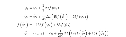
To save storage it is advantageous to compute ψN from the intermediate solutions ψ1 and ψ2 and combine the local tendencies in one array after the second substep (therefore low-storage scheme) as follows:
For reasons of clarity the time integration for several schemes (further schemes are: Leapfrog, Euler and 2nd order Runge-Kutta scheme) is implemented as follows (here e.g. the u-component of velocity):
u_p(k,j,i) = ( 1.0 - tsc(1) ) * u_m(k,j,i) + tsc(1) * u(k,j,i) + dt_3d * (
               tsc(2) * tend(k,j,i) + tsc(3) * tu_m(k,j,i)
             + tsc(4) * ( p(k,j,i) - p(k,j,i-1)) * ddx )
             - tsc(5) * rdf(k) * ( u(k,j,i) -ug )
and steered by the array tsc(1:5)
| tsc(1) | tsc(2) | tsc(3) | tsc(4) | tsc(5) | |
| 1 | 1/3 | 0 | 0 | 0 | 1st substep |
| 1 | 15/16 | -25/48 | 0 | 0 | 2nd substep |
| 1 | 8/15 | 1/15 | 0 | 1 | 3rd substep |
u_p is the prognosticated and u the current velocity at each substep. u_m denotes the velocity of the previous substep (needed for Leapfrog). tend is the current tendency and tu_m the combined tendencies of the prior substeps. tsc(4) steers the preconditioning of the pressure solver and tsc(5) the rayleigh damping.
References 
- Baldauf, M., 2008: Stability analysis for linear discretisations of the advection equation with Runge-Kutta time integration. J. Comput. Phys., 227, 6638-6659.
- Durran, D. R., 1999: Numerical methods for wave equations in geophysical fluid dynamics. Springer Verlag, New York, 1. Aufl., 465 S.
- Williamson, J. H., 1980: Low-storage Runge-Kutta schemes. J. Comput. Phys., 35, 48-56.