Home

Context Navigation

Version 53 (modified by suehring, 6 years ago) (diff)
--

Boundary conditions

Basics

PALM offers a variety of boundary conditions. Dirichlet or Neumann boundary conditions can be chosen for u, v, θ, q_v, and p^∗ at the bottom and top of the model. For the horizontal velocity components the choice of Neumann (Dirichlet) boundary conditions yields free-slip (no-slip) conditions. Neumann boundary conditions are also used for the SGS-TKE. Kinematic fluxes of heat and moisture can be prescribed at the surface instead (Neumann conditions) of temperature and humidity (Dirichlet conditions). At the top of the model, Dirichlet boundary conditions can be used with given values of the geostrophic wind. By default, the lowest grid level (k = 0) for the scalar quantities and horizontal velocity components is not staggered vertically and defined at the surface (z = 0). In case of free-slip boundary conditions at the bottom of the model, the lowest grid level is defined below the surface (z = - 0.5 Δz) instead. Vertical velocity is assumed to be zero at the surface and top boundaries, which implies using Neumann conditions for pressure.

Following Monin-Obukhov similarity theory (MOST) a constant flux layer can be assumed as boundary condition between the surface and the first grid level where scalars and horizontal velocities are defined (k = 1, z_MO = 0.5 Δz). It is then required to provide the roughness lengths for momentum z₀ and heat z_0,h. Momentum and heat fluxes as well as the horizontal velocity components are calculated using the following framework. The formulation is theoretically only valid for horizontally-averaged quantities. In PALM we assume that MOST can be also applied locally and we therefore calculate local fluxes, velocities, and scaling parameters.

Following MOST, the vertical profile of the horizontal wind velocity

$\begin{equation*} u_\mathrm{h} = (u^2 + v^2)^{\frac{1}{2}} \end{equation*}$

is given in the surface layer by

$\begin{align*} & \frac{\partial u_\mathrm{h}}{\partial z} = \frac{u_\ast}{\kappa z}\Phi_\mathrm{m}\left(\frac{z}{L}\right)\;, \end{align*}$

where κ = 0.4 is the Von Kármán constant and Φ_m is the similarity function for momentum in the formulation of Businger-Dyer (see e.g. Panofsky and Dutton 1984)

$\begin{align*} & \Phi_\mathrm{m} = \begin{cases} 1 + 5 \frac{z}{L} & \text{for~} \frac{z}{L} \geq 0 \\ \left(1 - 16 \frac{z}{L}\right)^{-\frac{1}{4}} & \text{for~} \frac{z}{L} < 0\;. \end{cases} \end{align*}$

Here, L is the Obukhov length, calculated as

$\begin{align*} & L = \frac{\theta_\mathrm{v}(z) u_\ast^2}{\kappa g \left[\theta_\ast + 0.61 \theta(z) q_\ast + 0.61 q_\mathrm{v}(z) \theta_\ast\right]}\;. \end{align*}$

The scaling parameters θ_* and q_* are defined by MOST as:

$\begin{align*} & \theta_\ast = - \frac{\overline{w^{\prime\prime}\theta^{\prime\prime}}_0}{u_\ast},~q_\ast = - \frac{\overline{w^{\prime\prime}q_\mathrm{v}^{\prime\prime}}_0}{u_\ast}\;, \end{align*}$

with the friction velocity u_* defined as

$\begin{align*} & u_\ast = \left[\left(\overline{u^{\prime\prime} w^{\prime\prime}}_0\right)^2 + \left(\overline{v^{\prime\prime} w^{\prime\prime}}_0\right)^2 \right]^{\frac{1}{4}}\;. \end{align*}$

In PALM, u_* is calculated from u_h at z_MO by vertical integration over z from z₀ to z_MO.

From the equations above it is possible to derive a formulation for the horizontal wind components, viz.

$\begin{align*} & \frac{\partial u}{\partial z} = \frac{-\overline{u^{\prime\prime} w^{\prime\prime}}_0}{u_\ast \kappa z} \Phi_\mathrm{m}\left(\frac{z}{L}\right)\,\text{and~}\,\frac{\partial v}{\partial z} = \frac{-\overline{v^{\prime\prime} w^{\prime\prime}}_0}{u_\ast \kappa z} \Phi_\mathrm{m}\left(\frac{z}{L}\right)\;. \end{align*}$

Vertical integration over z from z₀ to z_MO of the equation above then yields the surface momentum fluxes

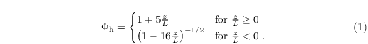
$\overline{u^{\prime\prime} w^{\prime\prime}}_0,\;\; \overline{v^{\prime\prime} w^{\prime\prime}}_0$

The formulations above all require knowledge of the scaling parameters θ_* and q_*. These are deduced from vertical integration of

$\begin{align} & \frac{\partial \theta}{\partial z} = \frac{\theta_\ast}{\kappa z} \Phi_\mathrm{h}\left(\frac{z}{L}\right)~{\text{and}}~\frac{\partial q_\mathrm{v}}{\partial z} = \frac{q_\ast}{\kappa z} \Phi_\mathrm{h}\left(\frac{z}{L}\right) \end{align}$

over z from z_0,h to z_MO. The similarity function Φ_h is given by

$\begin{align} & \Phi_\mathrm{h} = \begin{cases} 1 + 5 \frac{z}{L} & \text{for~} \frac{z}{L} \geq 0 \\ \left(1 - 16 \frac{z}{L}\right)^{-1/2} & \text{for~} \frac{z}{L} < 0\;. \end{cases} \end{align}$

Currently, there are three different options to calculate the Obukhov length and the surface fluxes which are steered via the NAMELIST parameter most_method.

Method 1: circular

The traditional implementation in PALM (most_method = 'circular') requires the use of data from the previous time step. The following steps are thus carried out in sequential order. First of all, θ_* and q_* are calculated by integration of the corresponding vertical derivation functions mentioned above using the value of z_MO/L from the previous time step. Second, the new value of z_MO/L is derived from the equation for L using the new values of θ_* and q_* but using u_* from the previous time step. Then, the new values of u_*, and subsequently the momentum fluxes are calculated by integration, respectively. At last, the above equations for the scaling parameters are employed to calculate the new surface fluxes by using θ_* and q_*, and u_*. In the special case, when surface fluxes are prescribed instead of surface temperature and humidity, the first and last steps are omitted and θ_* and q_* are directly calculated from u_* and the surface fluxes.

In summary, the following actions are performed in sequential order:

calculate θ_* and q_*
calculate u_h
determine Obukhov length
calculate u_*
derive surface fluxes

Method 2: Newton iteration / lookup table

Alternatively, the Obukhov length can be calculated by solving an implicit equation relating the L to the bulk Richardson number. This can be achieved either by a Newton iteration algorithm (most_method = 'newton') or by using a lookup table (most_method = 'lookup'). Note that the latter is faster than the Newton iteration method and the results of both methods are more precise compared to the circular method. However, it can only be used when the roughness lengths are homogeneously set on each processor.

Both methods require a different sequential order to derive the surface fluxes:

calculate u_h
determine Obukhov length (Newton iteration or lookup table)
calculate u_*
calculate θ_* and q_*
derive surface fluxes

Depending on whether Neumann (prescribed fluxes) or Dirichlet boundary conditions are used for temperature and humidity, the bulk Richardson number is related to the Obukhov length via

$\begin{equation*} Ri_\mathrm{b,Di} = \dfrac{z}{L} \cdot \dfrac{[\phi_\mathrm{H}]}{[\phi_\mathrm{M}]^2} \;\;\;\;\textnormal{(Dirichlet conditions)} \end{equation*} \begin{equation*} Ri_\mathrm{b,Ne} = \dfrac{z}{L} \cdot \dfrac{1}{[\phi_\mathrm{M}]^3} \;\;\;\;\textnormal{(Neumann conditions)} \end{equation*}$

where

$\begin{equation*} [\phi_\mathrm{H}] = \log\left(\dfrac{z_\mathrm{MO}}{z_\mathrm{0,h}}\right) - \Phi_\mathrm{H}\left(\dfrac{z_\mathrm{MO}}{L}\right) + \Phi_\mathrm{H}\left(\dfrac{z_\mathrm{0,h}}{L}\right)\;, \end{equation*} \begin{equation*} [\phi_\mathrm{M}] = \log\left(\dfrac{z_\mathrm{MO}}{z_\mathrm{0}}\right) - \Phi_\mathrm{M}\left(\dfrac{z_\mathrm{MO}}{L}\right) + \Phi_\mathrm{M}\left(\dfrac{z_\mathrm{0,h}}{L}\right)\;, \end{equation*}$

are the integrated universal profile stability functions of Φ_m and Φ_h (see Paulson 1970, Holtslag and Bruin 1988), and

$\begin{equation*} Ri_\mathrm{b,Di} = \dfrac{g z_\mathrm{MO} \left(\theta_\mathrm{v,1} - \theta_\mathrm{v,0}\right)}{u_\mathrm{h}^2 \theta_v}\;, \end{equation*} \begin{equation*} Ri_\mathrm{b,Ne} = - \dfrac{g z_\mathrm{MO} \overline{w^{\prime\prime} \theta_\mathrm{v}^{\prime\prime}}_0}{\kappa^2 u_\mathrm{h}^3 \theta_v}\;. \end{equation*}$

In case of most_method = 'newton', the above equations are solved for L by Newton iteration, i.e. finding the root of the equation

$\begin{equation*} f = Ri_\mathrm{b} - \dfrac{z}{L} \cdot \dfrac{[\phi_\mathrm{H}]^x}{[\phi_\mathrm{M}]^y} \end{equation*}$

where x and y depend on the chosen boundary conditions (see above). The solution is given by iteration of

$\begin{equation*} L^{t+1} = L^t - \dfrac{f(L^t)}{f'(L^t)} \end{equation*}$

with

$\begin{equation*} f'(L) = \dfrac{df}{dL} \end{equation*}$

until L meets a convergence criterion.

If most_method = 'lookup' is used, a table of Ri_b against z_MO/L is created at model start, based on the prescribed values of the roughness lengths. During the model run, Ri_b is calculated and the respectively value of z_MO/L is retrieved from the lookup table and using linear interpolation between the discrete values in the table. In order to speed up this method, the value of Ri_b from the previous time step is used as initial value. Due to the fact that the lookup table is created at model start, it is essential that the roughness lengths are 1) homogeneous on each processor (limiting this method to homogeneous surface configurations) and should not vary during the simulation (should thus not be used when using dynamic roughness length over water surfaces). For more details, see surface_layer_fluxes.f90.

Furthermore, the flat bottom of the model can be replaced by a Cartesian topography (see Sect. Topography).

By default, lateral boundary conditions are set to be cyclic in both directions. Alternatively, it is possible to opt for non-cyclic conditions in one direction, i.e., a laminar or turbulent inflow boundary (see Sect. Laminar and turbulent inflow boundary conditions) and an open outflow boundary on the opposite site (see Sect. Open outflow boundary conditions). The boundary conditions for the other direction have to remain cyclic. A complete overview about the non-cyclic lateral boundary conditions is given in Sect. non-cyclic lateral boundary conditions

In order to prevent gravity waves from being reflected at the top boundary, a sponge layer (Rayleigh damping) can be applied to all prognostic variables in the upper part of the model domain (Klemp and Lilly, 1978). Such a sponge layer should be applied only within the free atmosphere, where no turbulence is present.

The model is initialized by horizontally homogeneous vertical profiles of potential temperature, water vapor mixing ratio (or a passive scalar), and the horizontal wind velocities. The latter can be also provided from a 1-D precursor run (see Sect.1-D model for precursor runs). Uniformly distributed random perturbations with a user-defined amplitude can be imposed to the fields of the horizontal velocities components to initiate turbulence.

Laminar and turbulent inflow boundary conditions

In case of laminar inflow, Dirichlet boundary conditions are used for all quantities, except for the SGS-TKE e and perturbation pressure π^∗ for which Neumann boundary conditions are used. Vertical profiles, as taken for the initialization of the simulation, are used for the Dirichlet boundary conditions. In order to allow for a fast turbulence development, random perturbations can be imposed on the velocity fields within a certain area behind the inflow boundary (inlet). These perturbations may persist for the entire simulation. For the purpose of preventing gravity waves from being reflected at the inlet, a relaxation area can be defined after Davies (1976). So far, it was found to be sufficient to implement this method for temperature only. This is hence realized by an additional term in the prognostic equation for θ (see third equation in Sect. governing equation):

$\begin{align*} \frac{\partial \theta}{\partial t} = \ldots - C_{\text{relax}} \left(\theta - \theta_{\text{inlet}}\,\right). \end{align*}$

Here, θ_inlet is the stationary inflow profile of θ, and C_relax is a relaxation coefficient, depending on the distance d from the inlet, viz.

$\begin{align*} &C_{\text{relax}}(d) = \begin{cases} F_{\text{inlet}} \cdot \sin^2 \left(\frac{\pi}{2} \frac{D - d}{D} \right) & \text{for~} d < D,\\ 0 & \text{for~} d \ge D,\\ \end{cases} \end{align*}$

with D being the length of the relaxation region and F_inlet being a damping factor. For more information about the inflow boundary see Sect. inflow boundary.

Turbulence recycling

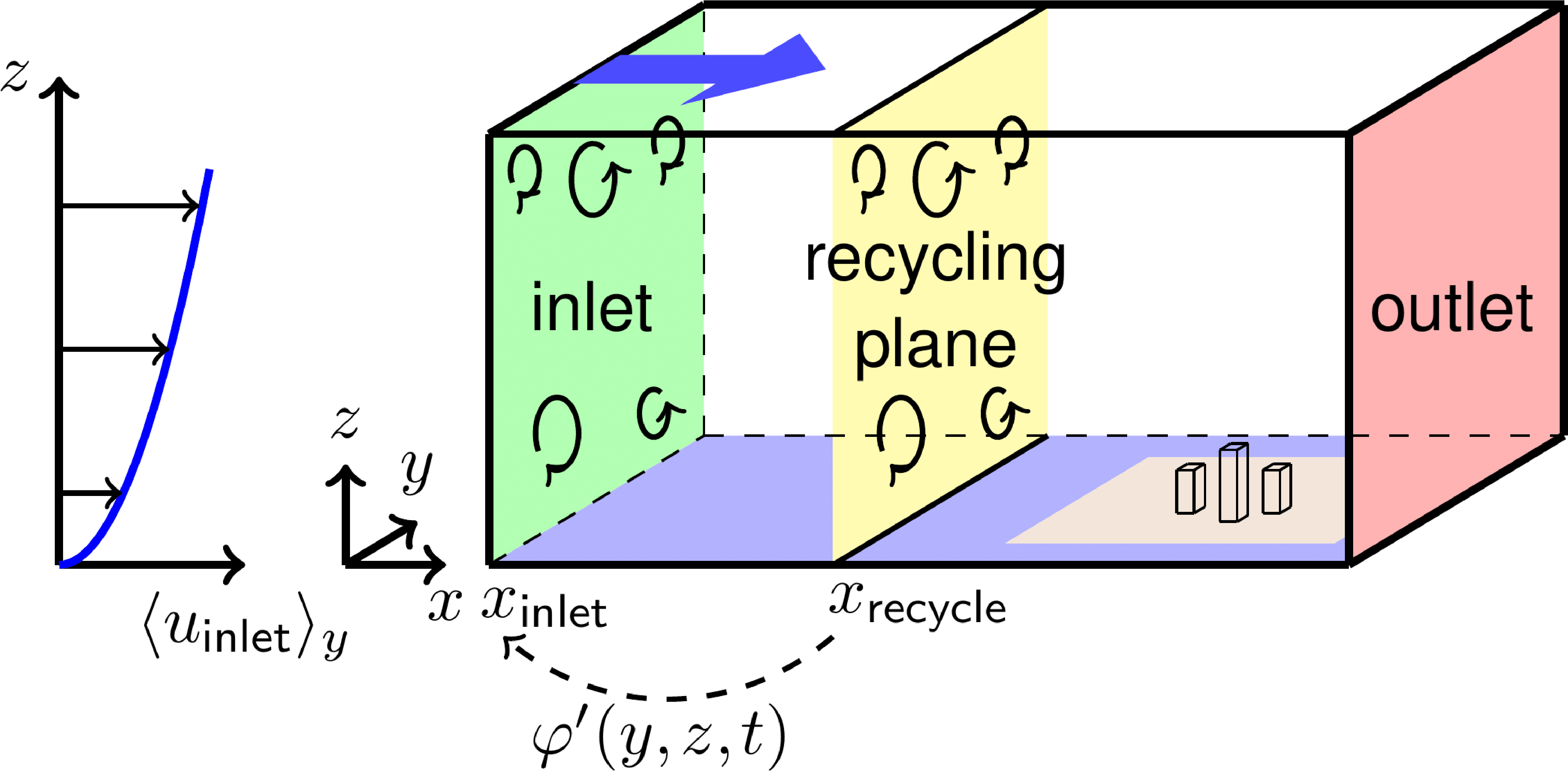
If non-cyclic horizontal boundary conditions are used, PALM offers the possibility of generating time-dependent turbulent inflow data by using a turbulence recycling method. The method follows the one described by Lund et al. (1998), with the modifications introduced by Kataoka and Mizuno (2002). Figure 2 gives an overview of the recycling method used in PALM.

Figure 3: Schematic figure of the turbulence recycling method used for generation of turbulent inflow. The configuration represents exemplary conditions with a built-up analysis area (brown surface) and an open water recycling area (blue surface). The blue arrow indicates the flow direction.

The turbulent signal φ^'(y, z, t) is taken from a recycling plane which is located at a fixed distance x_recycle from the inlet:

$\begin{align*} & \varphi^{\prime}(y, z, t) = \varphi(x_{\text{recycle}},y, z, t) - \langle \varphi\rangle_y(z, t), \end{align*}$

where <φ>_y(z, t) is the line average of a prognostic variable φ ∈ {u, v, w, θ, e} along y at x = x_recycle. φ^'(y, z, t) is then added to the mean inflow profile <φ_inflow>_y(z) at x_inlet after each time step:

$\begin{align*} & \varphi_{\text{inlet}}(y, z, t) = \langle \varphi_{\text{inlet}}\rangle_y(z) + \phi(z) \varphi^{\prime}(y, z, t), \end{align*}$

with the inflow damping function Φ(z), which has a value of 1 below the initial boundary layer height, and which is linearly damped to 0 above, in order to inhibit growth of the boundary layer depth. <φ_inlet>_y(z) is constant in time and either calculated from the results of the precursor run or prescribed by the user. The distance x_recycle has to be chosen much larger than the integral length scale of the respective turbulent flow. Otherwise, the same turbulent structures could be recycled repeatedly, so that the turbulence spectrum is illegally modified. It is thus recommended to use a precursor run for generating the initial turbulence field of the main run. The precursor run can have a comparatively small domain along the horizontal directions. In that case the domain of the main run is filled by cyclic repetition of the precursor run data. Note that the turbulence recycling has not been adapted for humidity and passive scalars so far.

Turbulence recycling is frequently used for simulations with urban topography. In such a case, topography elements should be placed sufficiently downstream of x_recycle to prevent effects on the turbulence at the inlet.

Synthetic Turbulence Generator

Since r2259 a synthetic turbulence generator is implemented in PALM to generate a turbulent inflow condition. The method is based on the work of Xie and Castro (2008) and Kim et al. (2013). Unscaled turbulent motions u_*j are computed based on length scales along each direction and the amplitude tensor a_ij which in turn bases on the Reynolds stress tensor. The calculated turbulence is then added to the mean inflow data of the velocity components U_i:

$\begin{equation*} u_i = U_i + a_{ij} u_{*j}. \end{equation*}$

The amplitude tensor a_ij depends on the Reynolds stress tensor R_ij and is calculated using a Cholesky decomposition as suggested by Lund et al. (1998). The unscaled turbulent motions u_*j, which are calculated on the 2D inflow plane, depend on the prescribed time scales t_ij and length scales l_ij:

$\begin{equation*} u_{*i}(t+\Delta t) = u_{*i}(t) \exp\left(-\dfrac{C\Delta t}{T}\right) + \Psi_i(t,L)\left[1-\exp\left(-\dfrac{2C\Delta t}{T}\right)\right]^{0.5}, \end{equation*}$

where Ψ denotes a part of the generated 2D signal which is correlated in space using the turbulent length scales l_ij along the vertical and spanwise direction. Correlation along streamwise direction is assured via the time scale t_ij which is estimated by t_ij along streamwise direction using the U_i.

After adding the turbulence to the mean inflow profiles, a mass flux correction suggested by Kim et al. (2013) is performed:

$\begin{equation*} u_{i,c} = \dfrac{U_{b,p}}{U_b} u_i, \end{equation*}$

where

$\begin{equation*} U_{b} = \dfrac{\int_S dS u_n}{S}, \end{equation*}$

where u_i,c is the corrected wind velocity at the inflow boundary, U_b and U_b,p the instantaneous and prescribed bulk velocity at the inflow boundary, S the surface area of the inflow boundary, and u_n the component of u_i normal to the inflow boundary.

The required length- and time scales, as well as the Reynolds strees tensor can be either prescribed (method 1), 0if known from previous simulations or measurements, or they can be parametrized (method 2). Please note, time and length scales as well as the components of the Reynolds stress tensor depend on the height and the horizontal location, particularly over heterogeneous surfaces and model domains with large horizontal extensions. For the sake of simplicity, however, we consider only height dependent information of the Reynolds stress as well as length and time scales.

Method 1: If these information is available, it can be provided via an ASCII file which contains all necessary information. For an example please see example file . This ASCII input file will be read automatically by PALM if the namelist parameter use_synthetic_turbulence_generator is set to True within the namelist stg_par. Be sure that the input file is added to the list of input files in your .palm.iofiles like so:

STG_PROFILES    in:locopt    d3#:d3r    $base_data/$fname/INPUT    _iprf

and named with the suffix _iprf in your INPUT directory. Please have look at the list of input and output files for a detailed description of the input file.

Method 2: In many cases detailed information about the Reynolds stress and turbulent length scales are not available, so that these information need to be parametrized. If no ASCII input file is provided in the input folder, this will be done automatically and the turbulence statistics at the inflow boundary will be estimated. Please note, the derived turbulence statistics will depend on the height above ground but not on the horizontal location. Parametrization of the Reynolds stress follows Rotach et al. (1996). The diagonal components R₁₁, R₂₂, indicating the horizontal velocity variances, are estimated as follows:

$\begin{equation*} R_{i,i} = u_{*}^2\,( 0.35\,(-\frac{z_i}{\kappa\,L})^\frac{2}{3} + (5 - 4\,\frac{z}{z_i}) )\,, \: (i \in (1,2)\,, \end{equation*}$

with u_* being the friction velocity, k the von-Kármán constant, L the Obukhov length, and z_i the mean boundary-layer depth. Please note, u_*, L and z_i are area-averaged values in this case. z describes the height of the respective model grid level. u_* is estimated from the mean horizontal wind speed at the first vertical grid point from the data provided at the lateral boundary using MOST. For the sake of simplicity, neutral conditions are assumed with Φ_m = 1. L is computed from the area-averaged surface temperature, sensible heat flux profile and roughness length in the model domain. z_i is estimated from the bulk Richardson criterion, with z_i being the height where the bulk Richardson first exceeds the critical Richardson number of 0.25, according to Heinze et al. (2017). In case of stable stratification (L > 0) or neutral stratification (L = 0), the first term is omitted for the computation of R_ii.
Further, vertical velocity variances are parametrized as

$\begin{equation*} R_{i,i} = w_{m}^2\,( 1.5\,(\frac{z}{z_i})^\frac{2}{3}\,e^(-2\,\frac{z}{z_i}) + (1.7 - \frac{z}{z_i})\,(\frac{u_{*}}{w_m})^2)\,, \: (i \in (3)\,, \end{equation*}$

with

$\begin{equation*} w_m = (u_{*}^{3} + 0.6\,w_{*}^{3})^\frac{1}{3} \end{equation*}$

being the momentum velocity scale, with the convective velocity scale w_*. In case of stable or neutral stratification, w_m = u_*. The remaining components R₃₁,R₃₂,R₂₁ are parametrized as

$\begin{equation*} R_{i,j} = u_{*}^2\,( 1 - e^(3\,\frac{z}{z_i} - 1))\,. \end{equation*}$

Too date, no proper parametrization of turbulent length scales that works for all stability regimes and within the entire boundary layer is available. Hence, for the moment the integral length scales are set to

TracMath macro processor has detected an error. Please fix the problem before continuing.

The command:

'/usr/bin/pdflatex -interaction=nonstopmode d91c6c508ea566ae0eb17a1677677c22b354bb28.tex'

failed with the following output:

"This is pdfTeX, Version 3.1415926-2.5-1.40.14 (TeX Live 2013)\n restricted \\write18 enabled.\nentering extended mode\n(./d91c6c508ea566ae0eb17a1677677c22b354bb28.tex\nLaTeX2e <2011/06/27>\nBabel <3.9h> and hyphenation patterns for 78 languages loaded.\n(/localdata/software/texlive/2013/texmf-dist/tex/latex/base/article.cls\nDocument Class: article 2007/10/19 v1.4h Standard LaTeX document class\n(/localdata/software/texlive/2013/texmf-dist/tex/latex/base/size10.clo))\n(/localdata/software/texlive/2013/texmf-dist/tex/latex/base/inputenc.sty\n(/localdata/software/texlive/2013/texmf-dist/tex/latex/base/utf8.def\n(/localdata/software/texlive/2013/texmf-dist/tex/latex/base/t1enc.dfu)\n(/localdata/software/texlive/2013/texmf-dist/tex/latex/base/ot1enc.dfu)\n(/localdata/software/texlive/2013/texmf-dist/tex/latex/base/omsenc.dfu)))\n(/localdata/software/texlive/2013/texmf-dist/tex/latex/cmap/cmap.sty)\n(/localdata/software/texlive/2013/texmf-dist/tex/latex/cm-super/type1ec.sty\n(/localdata/software/texlive/2013/texmf-dist/tex/latex/base/t1cmr.fd))\n(/localdata/software/texlive/2013/texmf-dist/tex/latex/base/fontenc.sty\n(/localdata/software/texlive/2013/texmf-dist/tex/latex/base/t1enc.def)<<t1.cmap\n>>) (/localdata/software/texlive/2013/texmf-dist/tex/latex/amsmath/amsmath.sty\nFor additional information on amsmath, use the `?' option.\n(/localdata/software/texlive/2013/texmf-dist/tex/latex/amsmath/amstext.sty\n(/localdata/software/texlive/2013/texmf-dist/tex/latex/amsmath/amsgen.sty))\n(/localdata/software/texlive/2013/texmf-dist/tex/latex/amsmath/amsbsy.sty)\n(/localdata/software/texlive/2013/texmf-dist/tex/latex/amsmath/amsopn.sty))\n(/localdata/software/texlive/2013/texmf-dist/tex/latex/amscls/amsthm.sty)\n(/localdata/software/texlive/2013/texmf-dist/tex/latex/amsfonts/amssymb.sty\n(/localdata/software/texlive/2013/texmf-dist/tex/latex/amsfonts/amsfonts.sty))\n(/localdata/software/texlive/2013/texmf-dist/tex/latex/tools/bm.sty)\n(/localdata/software/texlive/2013/texmf-dist/tex/latex/preview/preview.sty\n(/localdata/software/texlive/2013/texmf-dist/tex/latex/preview/prtightpage.def)\n)\nNo file d91c6c508ea566ae0eb17a1677677c22b354bb28.aux.\nPreview: Fontsize 10pt\nPreview: PDFoutput 1\n<<ot1.cmap>><<oml.cmap>><<oms.cmap>><<omx.cmap>>\n(/localdata/software/texlive/2013/texmf-dist/tex/latex/amsfonts/umsa.fd)\n(/localdata/software/texlive/2013/texmf-dist/tex/latex/amsfonts/umsb.fd)\n! Undefined control sequence.\nl.15 l_{i,j} = 8\\cdot \\MIN\n                          ( \\Delta x_i ) , \\: i \\in (1,2,3)\\,,\nPreview: Tightpage -32891 -32891 32891 32891\n[1{/localdata/software/texlive/2013/texmf-var/fonts/map/pdftex/updmap/pdftex.ma\np}] (./d91c6c508ea566ae0eb17a1677677c22b354bb28.aux) )\n(see the transcript file for additional information)</localdata/software/texliv\ne/2013/texmf-dist/fonts/type1/public/amsfonts/cm/cmmi10.pfb></localdata/softwar\ne/texlive/2013/texmf-dist/fonts/type1/public/amsfonts/cm/cmmi7.pfb></localdata/\nsoftware/texlive/2013/texmf-dist/fonts/type1/public/amsfonts/cm/cmr10.pfb></loc\naldata/software/texlive/2013/texmf-dist/fonts/type1/public/amsfonts/cm/cmsy10.p\nfb>\nOutput written on d91c6c508ea566ae0eb17a1677677c22b354bb28.pdf (1 page, 37822 b\nytes).\nTranscript written on d91c6c508ea566ae0eb17a1677677c22b354bb28.log.\n"

which arises from following considerations: On the one hand, from the numerical point of view the imposed perturbations should not be rapidly eliminated by the numerics. The numerical dissipation and dispersion, however, act on scales up to 8 time the grid spacing (5th order scheme, see: wiki:/doc/tec/discret]), meaning that scales < 8 times the grid spacing are rapidly dispersed and dissipated due to numerical errors. In order to trigger further turbulence development within the model domain, the imposed correlated turbulence should be on scales larger than the numerically-affected scales. On the other hand, however, imposing too large length scales could trigger structures that exist throughout the entire model domain, particularly under stable conditions, which in turn could bias the simulation results. Hence, as a compromise, length scales are set to 8 time the minimum grid spacing.

Note, for z>z_i the components of the stress tensor, length- and timescales are set to zero so that effectively no synthetic turbulence is imposed above the boundary-layer height (also saving computational costs). Please note, method 2 currently undergoes extensively testing.

At this point we emphasize that using the turbulence generator from Xie and Castro (2008) only generates turbulence which is correlated in space and time but not necessarily generate realistic turbulent structures as they occur in the real world. Large coherent structures such as e.g. hexagonal pattern as typically observed in a convective boundary layer, however, cannot be generated by this method. Further, we want to add that turbulence is only added to the three wind components. No perturbations are added to the subgrid-scale turbulent-kinetic energy and potential temperature.

If switched on, the turbulence generator imposed turbulent fluctuations on all lateral boundaries with Dirichlet boundary conditions for the velocity components. For example, if the offline nesting is switched on, where all four lateral boundaries are non-cyclic, the turbulence generator applied at all lateral boundaries, even though a lateral boundary is also an outflow boundary layer.

Open outflow boundary conditions

At the outflow boundary (outlet), the velocity components u_i meet radiation boundary conditions, viz.

$\begin{align*} \frac{\partial u_i}{\partial t} + U_{u_i} \frac{\partial u_i}{\partial n} = 0\,, \end{align*}$

as proposed by Orlanski (1976). Here ∂/∂n is the derivative normal to the outlet (i.e., ∂/∂x in Figure 2 and U_ui a transport velocity which includes wave propagation and advection. Rewriting the equation above yields the transport velocity

$\begin{align*} U_{u_i} = -\left(\frac{\partial u_i}{\partial t}\right)\left(\frac{\partial u_i}{\partial n}\right)^{-1} \end{align*}$

that is calculated at interior grid points next to the outlet at the preceding time step for each velocity component. If the transport velocity, calculated by means of the equation for the transport velocity, is outside the range 0 ≤ U_ui ≤ Δ/Δt, it is set to the respective threshold value that is exceeded. Because this local determination of U_ui can show high variations in case of complex turbulent flows, it is averaged laterally to the direction of the outflow, so that it varies only in the vertical direction. Alternatively, the transport velocity can be set to the upper threshold value (U_ui = Δ/Δt) for the entire outlet. Both equations mentioned in this section are discretized using an upstream method following Miller and Thorpe (1981). As the radiation boundary condition does not ensure conservation of mass, a mass flux correction can be applied at the outlet (see mass flux correction). For more information about the outflow boundary see Sect. outflow boundary.

Topography

The Cartesian topography in PALM is generally based on the mask method (Briscolini and Santangelo, 1989) and allows for explicitly resolving solid obstacles such as buildings and orography. The implementation makes use of the following simplifications:

the obstacle shape is approximated by (an appropriate number of) full grid cells to fit the grid, i.e., a grid cell is either 100% fluid or 100% obstacle,

the obstacles are fixed (not moving).

With revision -r2232, the topography implementation is completely revised. Starting from this revision, overhanging structures as for example bridges, ceilings, or tunnels, are allowed, i.e. topography does not necessarily be surface-mounted. If no overhanging structures are present, the 3-D obstacle dimension reduces to a 2.5-D topography format, which is conform to the Digital Elevation Model (DEM) format (DEMs of city morphologies have become increasingly available worldwide due to advances in remote sensing technologies). In case of overhanging structures, however, 3-D topography information is required to mask obstacles and their faces in PALM.

The model domain is then separated into three subdomains (see Fig. 3):

grid points in free fluid without adjacent surfaces, where the standard PALM code is executed,

grid points next to surface that require extra code (e.g., surface parametrization), and

grid points within obstacles, where the standard PALM code is executed but multiplied by zero.

Figure 4: Sketch of the topography implementation using the mask method (here for w). The yellow line represent the region where the prognostic terms for scalars and the w-component are masked, while the red line indicates the region where special surface-bounded code is masked. Additional surface-bounded code is executed at grid points in between the yellow and the red line (see topography implementation).

Additional topography code is executed in grid volumes of subdomain B. The faces of the obstacles are always located where the respective surface-normal velocity components u, v, and w are defined (cf. Fig. 1 in Sect. discretization) so that the impermeability boundary condition can be implemented by setting the respective surface-normal velocity component to zero.

In case of 5th-order advection scheme, the numerical stencil at grid points adjacent to obstacles would require data which is located within the obstacle. In order to avoid this, the order of the advection scheme is successively degraded at respective grid volumes adjacent to obstacles, i.e., from the 5th-order to 3rd-order at the second grid point above/beside an obstacle and from 3rd-order to 1st-order at grid points directly adjacent to an obstacle.

Surfaces in PALM can be aligned horizontally upward facing (e.g. bottom surface or rooftop), horizontally downward facing (e.g. undersurface of bridges), or vertically (facing north, east, south or west direction). At horizontal surfaces, PALM allows to either specify the surface values (θ, q_v, s) or to prescribe their respective surface fluxes. The latter is the only option for vertically oriented surfaces. Simulations with topography require the application of MOST between each surface and the first computational grid point outside of the topography. For vertical and horizontal downward-facing surfaces, neutral stratification is assumed for MOST, even if MOST is strictly speaking derived only for upward-facing horizontal surfaces. This is simply attributed to the lack of knowledge in the literature about the best practice in this matter.

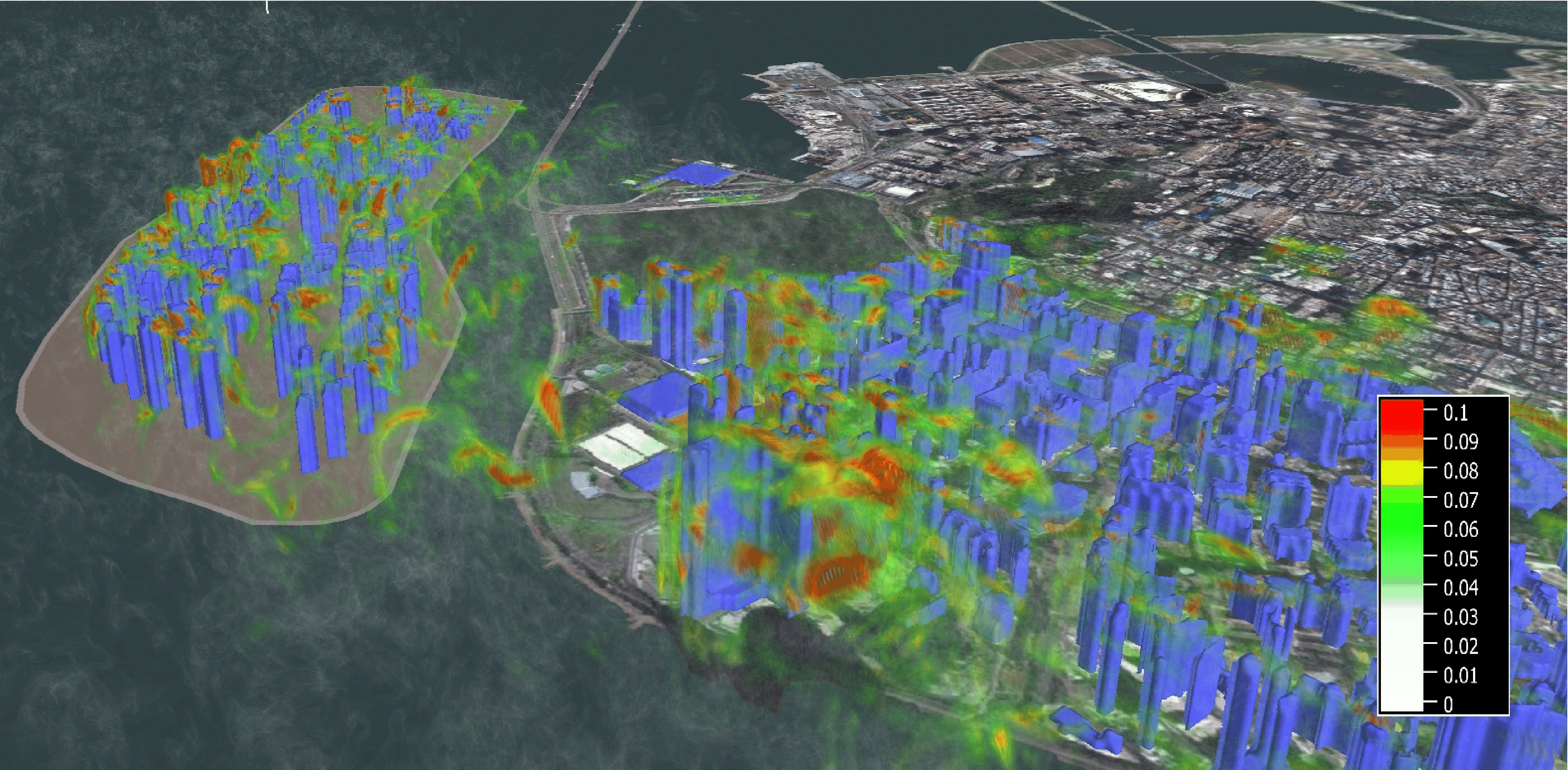
The topography implementation has been validated by Letzel et al. (2008) and Kanda et al. (2013). Park and Baik (2013) have recently extended the vertical wall boundary conditions for non-neutral stratifications and validated their results against wind tunnel data. Up to now, however, these modifications are not included in PALM 4.0. Figure 4 shows exemplarily the development of turbulence structures induced by a densely built-up artificial island off the coast of Macau, China (see also animation in Knoop et al., 2014). The approaching flow above the sea exhibits relatively weak turbulence due to the smooth water surface. Within the building areas, strong turbulence is generated by additional wind shear (due to the walls of isolated buildings) and due to a general increase in surface roughness.

Figure 5: Snapshot of the absolute value of the 3-D rotation vector of the velocity field (red to white colors) for a simulation of the city of Macau, including a newly built-up artificial island (left). Buildings are displayed in blue. A neutrally-stratified flow was simulated with the mean flow direction from the upper-left to the bottom-right, i.e. coming from the open sea and flowing from the artificial island to the city of Macau. The figure shows only a subregion of the simulation domain that spanned a horizontal model domain of about 6.1x2.0x1 km³, and with an equidistant grid spacing of 8m}$. The copyright for the underlying satellite image is held by Cnes / Spot Image, Digitalglobe. For more details, see associated animation Knoop et al. (2014).

The technical realization of the topography and treatment of surface-bounded grid cells will be outlined in Sect. topography implementation.

Non-cyclic lateral boundary conditions

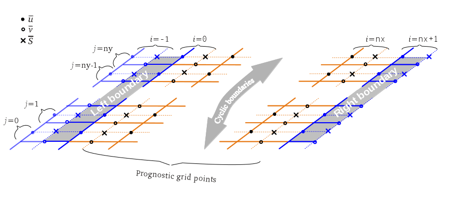
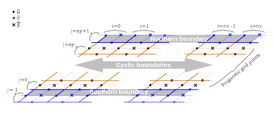
Figure 6 shows the grid structure for non-cyclic boundary conditions at the left/right boundary LB/RB (bc_lr) and figure 7 for non-cyclic boundary conditions at the north/south boundary NB/SB (bc_ns). The indices (i,j,k) represent the directions (x,y,z). The model domain extends from -1:nx+1 in the x-direction, from -1:ny+1 in the y-direction and from 0:nzt+1 in the z-direction. For the advection scheme of Wicker and Skamarock, two more grid points are added at the lateral boundaries which are not needed for non-cyclic boundary conditions. The figures display the grid layer of the horizontal velocity components u and v, and scalar s. The grid points of the vertical velocity w are defined at the scalar position but shifted by one half grid spacing in vertical direction (not shown, detailed information about the grid structure in PALM can be found here). The prognostic equations are solved at all inner grid points which are marked black. The grid points at the respective non-cyclic boundaries (blue) are treated as follows. LB is defined at i = -1 for v, w, s and at i = 0 for u. SB is defined at j = -1 for u, w, s and at j = 0 for v. RB is defined at i = nx + 1 and NB at j = ny + 1 for all quantities. LB and SB are treated this way so that the order and number of grid points for the streamwise velocity component and scalars is the same, independent of the flow direction.

For technical reasons, the prognostic equations are first solved for u at i = 0 (v at j = 0), since these grid points technically belong to the inner grid, but afterwards, these results at i = 0 (j = 0) are replaced by the respective boundary condition in routine boundary_conds.f90. In case of a Dirichlet condition, the values at i = 0 (j = 0) are taken from i = -1 (j = -1). In case of a radiation boundary condition, the solution of the Sommerfeld equation overwrites the prognostic values at i = 0 (j = 0).

For non-cyclic lateral boundary conditions, the parameter psolver has to be set to 'multigrid' because the default FFT-solver can only be applied for cyclic boundary conditions.

Figure 6: Grid structure at the lateral boundaries with non-cyclic lateral boundary conditions along the left-right direction.

Figure 7: Grid structure of the lateral boundaries with non-cyclic lateral boundary conditions along the north-south direction.

Inflow boundary

At the inflow boundary, Dirichlet conditions are used for the three velocity components ψ = {u,v,w} as well as for all scalar quantities s and are implemented as follows (here e.g. for s and a flow in positive x direction):

$\begin{align*} s^{t + \Delta t}(k,j,-1) = s_{init}(k) \; . \end{align*}$

t denotes the time, Δt the time step and s_init the initialization profile of the scalar quantities which is constant in time. The quantities at the inflow are set by the initial vertical profiles (see initializing_actions). A Neumann condition is used for the subgrid-scale turbulent kinetic energy e (here e.g. for a left-right flow):

$\begin{align*} e^{t + \Delta t}(k,j,-1) = e^{t + \Delta t}(k,j,0) \; . \end{align*}$

To prevent gravity waves from being reflected at the inflow, a relaxation term can be added to the prognostic equations for the potential temperature θ (Davies, 1976):

$\begin{align*} \theta^{t+1}(d) = ... - \Delta t \cdot K(d) \cdot \left( \theta^{t}(d) - \theta_{init} \right) \; . \end{align*}$

Here, d is the distance normal to the wall and θ_init the initial value of the potential temperature, which corresponds to the value at the inflow boundary. The damping or relaxation function K depends only on the distance d to the inflow. K is calculated by

$\begin{align*} K(d) = \begin{cases} d_f \sin^2\left( \frac{\pi}{2} \frac{d_w - d}{d_w} \right) , \text{for } d < d_w \\ \qquad\quad 0 \qquad \quad \;\;\; , \text{for } d \ge d_w \end{cases} . \end{align*}$

d_f is a damping factor to control the damping intensity, and d_w is the width of the relaxation region extending from the inflow. Quantities d_f and d_w can be set with parameters pt_damping_factor and pt_damping_width, respectively. Both parameters have to be set by the user and must be adjusted case-by-case, because both parameters depend on the numerical and physical conditions, so that application of universal default values is not possible. So far, we have experience with gravity waves in case of cold air outbreaks, which grow in amplitude up to quite extreme values, if no damping is applied. In the respective simulations, we used typical values for pt_damping_factor of 0.05 and for pt_damping_width of 25 km in order to prevent the gravity waves from growing.

Outflow boundary

At the outflow, an open boundary condition is needed to ensure that disturbances of the mean flow can exit the model domain without effecting the flow upstream. For the scalar quantities, Neumann boundary conditions are used at the outflow boundary which is the simplest way. For the velocity components, a Neumann condition would require to be considered in the solution of the Poisson equation for perturbation pressure, which has not been realized so far, because it requires some technical effort. Instead, PALM offers two types of radiation boundary conditions for the velocity components, which are not in conflict with the pressure solver (see use_cmax, bc_lr and bc_ns). For the radiation condition, the Sommerfeld radiation equation is solved at the outflow

$\begin{align*} \partial_t \psi + c_{\psi} \partial_n \psi = 0 \; , \end{align*}$

which considers flow disturbances propagating with the mean flow and by waves. Here ψ is the transported quantity and ∂_n is the derivative normal to the outflow boundary. In PALM, based on the equation above, the radiation boundary condition is realized in two ways as follows.

Variable Phase velocity

The phase velocity c_ψ (also called convective velocity) is calculated after Orlanski (1976):

$\begin{align*} c_{\psi} = - \dfrac{\partial_t \psi}{\partial_n \psi} \; . \end{align*}$

If the outflow is defined at the right boundary (i = nx + 1, Left-right flow, see Fig. 6), the phase velocity for each velocity component is calculated by

$\begin{align*} c_{\psi} = - c_{max} \dfrac{\psi^t_{nx} - \psi^{t - \Delta t}_{nx} }{ \psi^{t-\Delta t}_{nx} - \psi^{t - \Delta t}_{nx-1} } \; , \end{align*}$

with the maximum phase velocity

$\begin{align*} c_{max} = \dfrac{\Delta x}{\Delta t} \; . \end{align*}$

The phase velocity has to be in the range of 0 ≤ c_ψ < c_max because negative values propagate waves back to the inner domain. c_max represents the maximum phase velocity that ensures numerical stability (Courant-Friedrichs-Lewy condition). Both conditions are not ensured by the second equation of c_ψ, hence c_ψ is set to zero for negative values and to c_max for larger values than c_max. The velocity components ψ at the outflow boundary are then calculated by

$\begin{align*} \psi^{t+\Delta t}_{nx+1} = \psi^{t}_{nx+1} - \dfrac{\overline{c}_{\psi}}{c_{max}} (\psi^{t}_{nx+1} - \psi^{t}_{nx}) \; , \end{align*}$

with the phase velocity averaged parallel to the outflow:

$\begin{align*} \overline{c}_{\psi} = \dfrac{1}{ny+1} \sum_{j=0}^{ny} c_{\psi, j} \; . \end{align*}$

In Orlanskis work, the phase velocity c_ψ was not averaged along the outflow, which is sufficient for simplified flows as shown by Yoshida and Watanabe (2010). However, we found that in simulations of shear driven convective boundary layer with a strong wind component along the outflow, the approach of Orlanski (1976) was unstable. Raymond and Kuo (1984) argued that locally calculated phase velocities leads to a large variation of phase speeds which can lead to numerical instabilities. Other works used a constant phase velocity or an average over the whole outflow area (see e.g. Fröhlich 2006, p.216) instead of the approach of Orlanski (1976). With this in mind, we tested the average phase velocity calculated from the last mentioned equation, and the solution at the outflow becomes stable. We did not additionally average the phase velocity along the vertical direction, because the background wind usually varies with height.

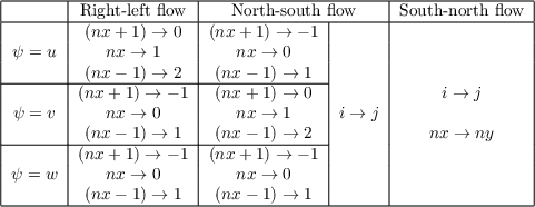
For the other flow directions, the indices of the above equations have to be replaced as follows:

$\begin{tabular}{|c |c |c |c| c|} \hline & Right-left flow & \multicolumn{2}{c|}{ North-south flow} & South-north flow \\ \hline & $(nx + 1) \rightarrow 0$ & $(nx + 1) \rightarrow -1$ & & \\ $\psi = u$ & $ nx \rightarrow 1$ & $ nx \rightarrow 0$ & & \\ & $(nx - 1) \rightarrow 2$ & $(nx - 1) \rightarrow 1$ & & \\ \cline{1-3} & $(nx + 1) \rightarrow -1$ & $(nx + 1) \rightarrow 0$ & & $i \rightarrow j$ \\ $\psi = v$ & $ nx \rightarrow 0$ & $ nx \rightarrow 1$ & $i \rightarrow j$ & \\ & $(nx - 1) \rightarrow 1$ & $(nx - 1) \rightarrow 2$ & & $nx \rightarrow ny$ \\ \cline{1-3} & $(nx + 1) \rightarrow -1$ & $(nx + 1) \rightarrow -1$ & & \\ $\psi = w$ & $ nx \rightarrow 0$ & $ nx \rightarrow 0$ & & \\ & $(nx - 1) \rightarrow 1$ & $(nx - 1) \rightarrow 1$ & & \\ \hline \end{tabular}$

Constant Phase velocity

Setting c_ψ = c_max leads to a more simple radiation boundary condition (here e.g. for a left-right flow along positive x-direction):

$\begin{align*} \psi^{t + \Delta t}(k,j,nx+1) = \psi^{t}(k,j,nx) \; , \end{align*}$

with ψ = {u,v,w}. This formulation of the radiation boundary condtions saves computational time compared to the formulation of a variable Phase velocity. Although, Orlanski (1976) suggested that this approach of radiation boundary condition leads to reflection for waves smaller than c_max which may occur in complex geophysical flows, our simulations of a convective boundary layer with background wind have been stable so far.

Mass flux correction

PALM offers the possibility of a mass flux correction at the outflow (e.g. Tian, 2004). If parameter conserve_volume_flow is set true, the mass flux at the inflow and outflow is calculated by:

$\begin{align*} \dot{m} = \sum_{k=1}^{nz-1} \Delta z(k) \sum_{l=0}^{nx_i} \psi(l,k) \Delta x_i \; . \end{align*}$

where Δx_i and ψ is equal to Δy (Δx) and u (v) in case of bc_lr (bc_ns). The correction factor for the outflow velocity, which is necessary due to different mass fluxes at inflow and outflow, can be calculated by

$\begin{align*} \psi_{corr} = \dfrac{\dot{m}_{inflow} - \dot{m}_{outflow}}{A} \; , \end{align*}$

where A is the area of the boundary

$\begin{align*} A = \sum_1^{nz-1} \Delta z \sum_0^{nx_i} \Delta x_i \; . \end{align*}$

The streamwise velocity at the outflow is corrected by adding ψ_corr at each grid point of the outflow between bottom and top (k=1:nz), in order to guarantee that the mass leaving the domain exactly balances the one entering it.

References

Holtslag AAM, Bruin HARD. 1988. Applied modelling of the night-time surface energy balance over land. J. Appl. Meteorol. 27: 689–704.

Panofsky HA, Dutton JA. 1984. Atmospheric Turbulence, Models and Methods for Engineering Applications. John Wiley & Sons. New York.

Paulson CA 1970. The mathematical representation of wind speed and temperature profiles in the unstable atmospheric surface layer. J. Appl. Meteorol. 9: 857–861.

Klemp JB, Lilly DK. 1978. Numerical simulation of hydrostatic mountain waves. J. Atmos. Sci. 35: 78–107.

Davies HC. 1976. A lateral boundary formulation for multi-level prediction models. Q. J. Roy. Meteor. Soc. 102: 405–418.

Lund TS, Wu X, Squires KD. 1998. Generation of turbulent inflow data for spatially-developing boundary layer simulations. J. Comput. Phys. 140: 233–258.

Kataoka H, Mizuno M. 2002. Numerical flow computation around aerolastic 3d square cylinder using inflow turbulence. Wind Struct. 5: 379–392.

Orlanski I. 1976. A simple boundary condition for unbounded hyperbolic flows. J. Comput. Phys. 21: 251–269.

Miller MJ, Thorpe AJ. 1981. Radiation conditions for the lateral boundaries of limited-area numerical models. Q. J. Roy. Meteor. Soc. 107: 615–628.

Xie ZT, Castro IP. 2008. Efficient generation of inflow conditions for large eddy simulation of street-scale flows. Flow, Turbul. Combust. 81: 449–470.

Kim Y, Castro IP, Xie ZT. 2013. Divergence-free turbulence inflow conditions for large-eddy simulations with incompressible flow solvers. Comput. Fluids. 84: 56–68

Rotach M, Gryning SE, Tassone C. 1996. A two-dimensional Lagrangian stochastic dispersion model for daytime condtions. Q.J.R. Meteorol. Soc. 122: 367–389.

Heinze R, Moseley C, Böske L, Muppa S, Maurer V, Raasch S. 2017. Evaluation of large-eddy simulations forced with mesoscale model output for a multi-week period during a measurement campaign. Atmos. Chem. Phys. 17: 7083-7109

Briscolini M, and Santangelo P. 1989. Development of the mask method for incompressible unsteady flows. J. Comput. Phys. 84: 57–75.

Letzel MO, Krane M, Raasch S. 2008. High resolution urban large-eddy simulation studies from street canyon to neighbourhood scale. Atmos. Environ. 42: 8770–8784.

Kanda M, Inagaki A, Miyamoto T, Gryschka M, Raasch S. 2013. A new aerodynamic parameterization for real urban surfaces. Bound.-Lay. Meteorol. 148: 357–377.

Park SB, and Baik J. 2013. A large-eddy simulation study of thermal effects on turbulence coherent structures in and above a building array. J. Appl. Meteorol. 52: 1348–1365.

Knoop H, Keck M, Raasch S. 2014. Urban large-eddy simulation - influence of a densely build-up artificial island on the turbulent flow in the city of Macau, Computer animation. doi.

Yoshida T, Watanabe T. 2010. Sommerfeld radiation condition for incompressible viscous flows. 5th European Conference on Computational Fluid Dynamics. 14-17 June. Lisbon, Portugal. ECCOMAS. 1-11.

Raymond WH, Kuo HL. 1984. A radiation boundary condition for multi-dimensional flows. Quart. J. R. Met. Soc. 110: 535–551.

Fröhlich F. 2006. Large eddy simulation turbulenter Strömungen. B.G. Teubner Verlag. 414 pp.

Tian W, Guo Z, Yu R. 2004. Treatment of LBCs in 2D simulation of convection over hills. Adv. Atmos. Sci. 21: 573–586.

Attachments (6)

03.png (465.4 KB) - added by Giersch 9 years ago. Turbulence recycling method
04.png (91.3 KB) - added by Giersch 9 years ago. Sketch of the 2.5-D implementation of topography
05.png (5.0 MB) - added by Giersch 9 years ago. Snapshot of turbulence structures induced by a densely built-up artificial island of the coast of Macau, China
grid_lr.png (89.4 KB) - added by Giersch 9 years ago. Grid structure at the lateral boundaries with non-cyclic lateral boundary conditions along the left-right direction
grid_ns.png (74.7 KB) - added by Giersch 9 years ago. Figure 2: Grid structure of the lateral boundaries with non-cyclic lateral boundary conditions along the north-south direction.
mask_method.png (19.6 KB) - added by suehring 8 years ago.

Download in other formats:

Plain Text