Home

Context Navigation

Version 2 (modified by Giersch, 9 years ago) (diff)
--

This site is currently under construction!

Ocean option

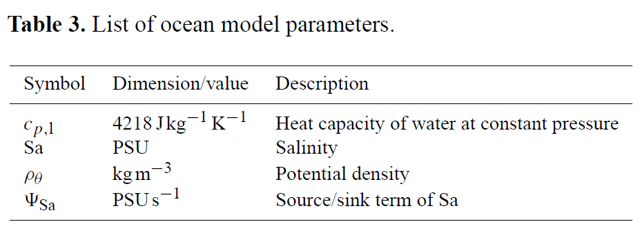
PALM allows for studying the ocean mixed layer (OML) by using an ocean option where the sea surface is defined at the top of the model, so that negative values of z indicate the depth. Hereafter, we keep the terminology and use the word surface and index 0 for variables at the sea surface and top of the ocean model. For a list of ocean specific parameters, see the following Table 3.

The ocean version differs from the atmospheric version by a few modifications, which are handled in the code by distinction of cases, so that both versions share the same basic code. In particular, seawater buoyancy and static stability depend not only on θ, but also on the salinity Sa. In order to account for the effect of salinity on density, a prognostic equation is added for Sa (in PSU, practical salinity unit):

$\begin{align*} \frac{\partial {\text{Sa}}}{\partial t} = - \frac{\partial u_j {\text{Sa}}}{\partial x_j} - \frac{\partial}{\partial x_j}\left(\overline{u_j^{\prime\prime}{\text{Sa}}^{\prime\prime}}\right) + \Psi_{\text{Sa}}\;, \end{align*}$

where Ψ_Sa represents sources and sinks of salinity. Furthermore, θ_v is replaced by potential density ρ_θ in the buoyancy term of the momentum equation (see Sect. governing equations)

$\begin{align*} + g \frac{\theta_\mathrm{v} - \langle\theta_{\mathrm{v}}\rangle}{\langle\theta_{\mathrm{v}}\rangle} \delta_{i3}\,\rightarrow\,- g \frac{\rho_{\theta} - \langle\rho_{\theta}\rangle}{\langle\rho_{\theta}\rangle} \delta_{i3}\;, \end{align*}$

in the stability-related term of the SGS-TKE equation (see Sect. turbulence closure)

$\begin{align*} + \frac{g}{\theta_{\mathrm{v},0}}\overline{u_3^{\prime\prime} {\theta_{\mathrm{v}}}^{\prime\prime}}\,\rightarrow\,+ \frac{g}{\rho_{\theta,0}}\overline{u_3^{\prime\prime} {\rho_{\theta}}^{\prime\prime}} \end{align*}$

as well as in the calculation of the mixing length (see Sect. turbulence closure)

$\begin{align*} & \left(\frac{g}{\theta_{\mathrm{v},0}} \frac{\partial{\theta_{\mathrm{v}}}}{\partial z}\right)^{-\frac{1}{2}}\,\rightarrow\,\left(\frac{g}{\rho_{\theta,0}} \frac{\partial{\rho_{\theta}}}{\partial z}\right)^{-\frac{1}{2}}\;. \end{align*}$

ρ_θ is calculated from the equation of state of seawater after each time step using the algorithm proposed by Jackett et al. (2006). The algorithm is based on polynomials depending on Sa, θ, and p (see Jackett et al., 2006, Table A2). At the moment, only the initial values of p enter this equation.
The ocean is driven by prescribed fluxes of momentum, heat and salinity at the top. The boundary conditions at the bottom of the model can be chosen as for atmospheric runs, including the possibility to use topography at the sea bottom.
Note that the current version of the ocean option does not account for the effect of surface waves (e.g., Langmuir circulation and wave-breaking). Parametrization schemes might, however, be provided within the user interface (see Sect. user interface) and have been used, e.g., by \citet{noh2004}. The ocean option in its current state was recently used for simulations of the ocean mixed layer by \citet{esau2014}, who investigated indirect air-sea interactions by means of the atmosphere-ocean coupling scheme that will be described in Sect. coupled atmosphere-ocean simulations. Note that most previous PALM studies of the OML used the atmospheric code, subsequent inversion of the z-axis and appropriate normalization of the results, instead of using the relatively new ocean option \citep[e.g.][]{noh2004,noh2009}.

References

Jackett DR, Mc Dougall TJ, Feistel R, Wright DG, Griffies SM. 2006. Algortihms for density, potential temperature, conservative temperature, and the freezing temperature of seawater. J. Atmos. Ocean. Tech. 23: 1709–1728.

Attachments (1)

Table3.png (23.8 KB) - added by Giersch 9 years ago. List of ocean model parameters

Download all attachments as: .zip

Download in other formats:

Plain Text