| Version 6 (modified by Giersch, 9 years ago) (diff) |
|---|
This site is currently under construction!
Cloud mircrophysics 
PALM offers an embedded bulk cloud microphysics representation that takes into account the liquid water specific humidity and warm (i.e., no ice) cloud-microphysical processes. Therefore, PALM solves the prognostic equations for the total water content

instead of qv, and for a linear approximation of the liquid water potential temperature (e.g., Emanuel, 1994)

instead of θ as described in Sect. governing equations. Since q and θl are conserved quantities for wet adiabatic processes, condensation/evaporation is not considered for these variables.
Liquid phase microphysics are parametrized following the two-moment scheme of Seifert and Beheng (2001,2006), which is based on the separation of the droplet spectrum into droplets with radii < 40 μm (cloud droplets) and droplets with radii ≥ 40 μm (rain droplets). The model predicts the first two moments of these partial droplet spectra, namely cloud and rain droplet number concentration (Nc and Nr, respectively) as well as cloud and rain water specific humidity (qc and qr, respectively). Consequently, ql is the sum of both qc and qr. The moments' corresponding microphysical tendencies are derived by assuming the partial droplet spectra to follow a gamma distribution that can be described by the predicted quantities and empirical relationships for the distribution's slope and shape parameters. For a detailed derivation of these terms, see Seifert and Beheng (2001,2006).
We employ the computational efficient implementation of this scheme as used in the UCLA-LES (Savic-Jovcic and Stevens, 2008) and DALES (Heus et al., 2010) models. We thus solve only two additional prognostic equations for Nr and qr:

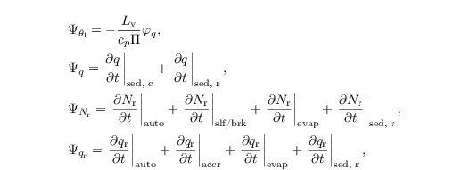
with the sink/source terms ΨNr and Ψqr, and the SGS fluxes

with Nc and qc being a fixed parameter and a diagnostic quantity, respectively.
In the next subsections we will describe the diagnostic determination of qc. From Sect. autoconversion on, the microphysical processes considered in the sink/source terms of θl, q, Nr and qr,

are used in the formulations of Seifert and Beheng (2006) unless explicitly specified. Section turbulence closure gives an overview of the necessary changes for the turbulence closure (cf. Sect. turbulence closure) using q and θl instead of qv and $θ$, respectively.
Diffusional growth of cloud water 
Autoconversion 
Accretion 
Self-collection and breakup 
Evaporation of rainwater 
Sedimentation of rainwater 
Turbulence closure 
Recent applications 
References 
- ¶Emanuel KA. 1994. Atmospheric Convection. Oxford University Press.
- ¶Seifert A, Beheng KD. 2001. A double-moment parameterization for simulating autoconversion, accretion and selfcollection. Atmos. Res. 59: 265–281.
- ¶Seifert A, Beheng KD. 2006. A two-moment cloud microphysics parameterization for mixed-phase clouds. Part 1: Model description. Meteorol. Atmos. Phys. 92: 45–66.
Attachments (8)
-
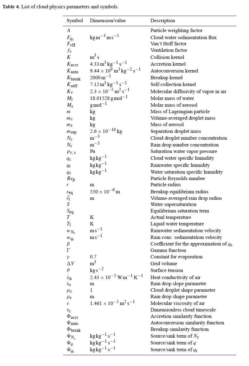
Table4.png
(114.2 KB) -
added by Giersch 9 years ago.
List of cloud physics parameters and symbols
-
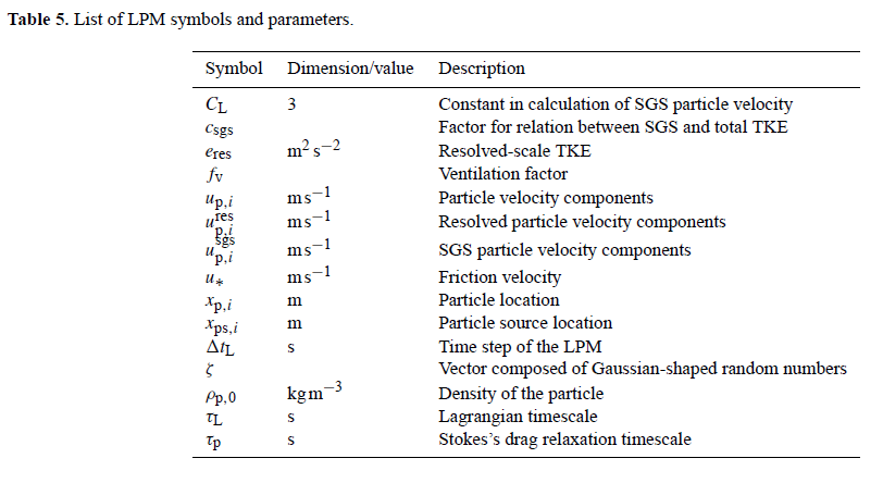
Table5.png
(38.6 KB) -
added by Giersch 9 years ago.
List of LPM symbols and parameters
-
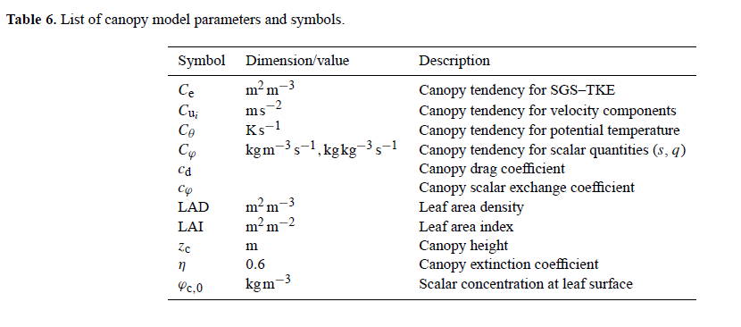
Table6.png
(32.0 KB) -
added by Giersch 9 years ago.
List of canopy model parameters and symbols
-
06.png
(3.0 MB) -
added by Giersch 9 years ago.
Snapshot of the cloud field from a PALM run for.
- Button_Example.png (56.3 KB) - added by westbrink 6 years ago.
- Button_InputPara.png (57.8 KB) - added by westbrink 6 years ago.
- Button_Overview.png (56.0 KB) - added by westbrink 6 years ago.
- Button_References.png (55.5 KB) - added by westbrink 6 years ago.


