Home

Context Navigation

Version 20 (modified by Giersch, 9 years ago) (diff)
--

This site is currently under construction!

Boundary conditions

Basics

PALM offers a variety of boundary conditions. Dirichlet or Neumann boundary conditions can be chosen for u, v, θ, q_v, and p^∗ at the bottom and top of the model. For the horizontal velocity components the choice of Neumann (Dirichlet) boundary conditions yields free-slip (no-slip) conditions. Neumann boundary conditions are also used for the SGS-TKE. Kinematic fluxes of heat and moisture can be prescribed at the surface instead (Neumann conditions) of temperature and humidity (Dirichlet conditions). At the top of the model, Dirichlet boundary conditions can be used with given values of the geostrophic wind. By default, the lowest grid level (k = 0) for the scalar quantities and horizontal velocity components is not staggered vertically and defined at the surface (z = 0). In case of free-slip boundary conditions at the bottom of the model, the lowest grid level is defined below the surface (z = - 0.5 Δz) instead. Vertical velocity is assumed to be zero at the surface and top boundaries, which implies using Neumann conditions for pressure.

Following Monin-Obukhov similarity theory (MOST) a constant flux layer can be assumed as boundary condition between the surface and the first grid level where scalars and horizontal velocities are defined (k = 1, z_MO = 0.5 Δz). It is then required to provide the roughness lengths for momentum z₀ and heat z_0,h. Momentum and heat fluxes as well as the horizontal velocity components are calculated using the following framework. The formulation is theoretically only valid for horizontally-averaged quantities. In PALM we assume that MOST can be also applied locally and we therefore calculate local fluxes, velocities, and scaling parameters.

Following MOST, the vertical profile of the horizontal wind velocity

$\begin{equation*} u_\mathrm{h} = (u^2 + v^2)^{\frac{1}{2}} \end{equation*}$

is given in the surface layer by

$\begin{align*} & \frac{\partial u_\mathrm{h}}{\partial z} = \frac{u_\ast}{\kappa z}\Phi_\mathrm{m}\left(\frac{z}{L}\right)\;, \end{align*}$

where κ = 0.4 is the Von Kármán constant and Φ_m is the similarity function for momentum in the formulation of Businger-Dyer (see e.g. Panofsky and Dutton 1984)

$\begin{align*} & \Phi_\mathrm{m} = \begin{cases} 1 + 5 \frac{z}{L} & \text{for~} \frac{z}{L} \geq 0 \\ \left(1 - 16 \frac{z}{L}\right)^{-\frac{1}{4}} & \text{for~} \frac{z}{L} < 0\;. \end{cases} \end{align*}$

Here, L is the Obukhov length, calculated as

$\begin{align*} & L = \frac{\theta_\mathrm{v}(z) u_\ast^2}{\kappa g \left[\theta_\ast + 0.61 \theta(z) q_\ast + 0.61 q_\mathrm{v}(z) \theta_\ast\right]}\;. \end{align*}$

The scaling parameters θ_* and q_* are defined by MOST as:

$\begin{align*} & \theta_\ast = - \frac{\overline{w^{\prime\prime}\theta^{\prime\prime}}_0}{u_\ast},~q_\ast = - \frac{\overline{w^{\prime\prime}q_\mathrm{v}^{\prime\prime}}_0}{u_\ast}\;, \end{align*}$

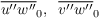
with the friction velocity u_* defined as

$\begin{align*} & u_\ast = \left[\left(\overline{u^{\prime\prime} w^{\prime\prime}}_0\right)^2 + \left(\overline{v^{\prime\prime} w^{\prime\prime}}_0\right)^2 \right]^{\frac{1}{4}}\;. \end{align*}$

In PALM, u_* is calculated from u_h at z_MO by vertical integration over z from z₀ to z_MO.

From the equations above it is possible to derive a formulation for the horizontal wind components, viz.

$\begin{align*} & \frac{\partial u}{\partial z} = \frac{-\overline{u^{\prime\prime} w^{\prime\prime}}_0}{u_\ast \kappa z} \Phi_\mathrm{m}\left(\frac{z}{L}\right)\,\text{and~}\,\frac{\partial v}{\partial z} = \frac{-\overline{v^{\prime\prime} w^{\prime\prime}}_0}{u_\ast \kappa z} \Phi_\mathrm{m}\left(\frac{z}{L}\right)\;. \end{align*}$

Vertical integration over z from z₀ to z_MO of the equation above then yields the surface momentum fluxes

$\overline{u^{\prime\prime} w^{\prime\prime}}_0,\;\; \overline{v^{\prime\prime} w^{\prime\prime}}_0$

The formulations above all require knowledge of the scaling parameters θ_* and q_*. These are deduced from vertical integration of

$\begin{align} & \frac{\partial \theta}{\partial z} = \frac{\theta_\ast}{\kappa z} \Phi_\mathrm{h}\left(\frac{z}{L}\right)~{\text{and}}~\frac{\partial q_\mathrm{v}}{\partial z} = \frac{q_\ast}{\kappa z} \Phi_\mathrm{h}\left(\frac{z}{L}\right) \end{align}$

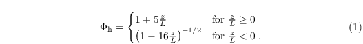
over z from z_0,h to z_MO. The similarity function Φ_h is given by

$\begin{align} & \Phi_\mathrm{h} = \begin{cases} 1 + 5 \frac{z}{L} & \text{for~} \frac{z}{L} \geq 0 \\ \left(1 - 16 \frac{z}{L}\right)^{-1/2} & \text{for~} \frac{z}{L} < 0\;. \end{cases} \end{align}$

Currently, there are three different options to calculate the Obukhov length and the surface fluxes which are steered via the NAMELIST parameter most_method.

Method 1: circular

The traditional implementation in PALM (most_method = 'circular') requires the use of data from the previous time step. The following steps are thus carried out in sequential order. First of all, θ_* and q_* are calculated by integration of the corresponding vertical derivation functions mentioned above using the value of z_MO/L from the previous time step. Second, the new value of z_MO/L is derived from the equation for L using the new values of θ_* and q_* but using u_* from the previous time step. Then, the new values of u_*, and subsequently the momentum fluxes are calculated by integration, respectively. At last, the above equations for the scaling parameters are employed to calculate the new surface fluxes by using θ_* and q_*, and u_*. In the special case, when surface fluxes are prescribed instead of surface temperature and humidity, the first and last steps are omitted and θ_* and q_* are directly calculated from u_* and the surface fluxes.

In summary, the following actions are performed in sequential order:

calculate θ_* and q_*
calculate u_h
determine Obukhov length
calculate u_*
derive surface fluxes

Method 2: Newton iteration / lookup table

Alternatively, the Obukhov length can be calculated by solving an implicit equation relating the L to the bulk Richardson number. This can be achieved either by a Newton iteration algorithm (most_method = 'newton') or by using a lookup table (most_method = 'lookup'). Note that the latter is the new default in PALM as it is much faster than the Newton iteration method and the results are more precise compared to the circular method. However, it can only be used when the roughness lengths are homogeneously set on each processor.

Both methods require a different sequential order to derive the surface fluxes:

calculate u_h
determine Obukhov length (Newton iteration or lookup table)
calculate u_*
calculate θ_* and q_*
derive surface fluxes

Depending on whether Neumann (prescribed fluxes) or Dirichlet boundary conditions are used for temperature and humidity, the bulk Richardson number is related to the Obukhov length via

$\begin{equation*} Ri_\mathrm{b,Di} = \dfrac{z}{L} \cdot \dfrac{[\phi_\mathrm{H}]}{[\phi_\mathrm{M}]^2} \;\;\;\;\textnormal{(Dirichlet conditions)} \end{equation*} \begin{equation*} Ri_\mathrm{b,Ne} = \dfrac{z}{L} \cdot \dfrac{1}{[\phi_\mathrm{M}]^3} \;\;\;\;\textnormal{(Neumann conditions)} \end{equation*}$

where

$\begin{equation*} [\phi_\mathrm{H}] = \log\left(\dfrac{z_\mathrm{MO}}{z_\mathrm{0,h}}\right) - \Phi_\mathrm{H}\left(\dfrac{z_\mathrm{MO}}{L}\right) + \Phi_\mathrm{H}\left(\dfrac{z_\mathrm{0,h}}{L}\right)\;, \end{equation*} \begin{equation*} [\phi_\mathrm{M}] = \log\left(\dfrac{z_\mathrm{MO}}{z_\mathrm{0}}\right) - \Phi_\mathrm{M}\left(\dfrac{z_\mathrm{MO}}{L}\right) + \Phi_\mathrm{M}\left(\dfrac{z_\mathrm{0,h}}{L}\right)\;, \end{equation*}$

are the integrated universal profile stability functions of Φ_m and Φ_h (see Paulson 1970, Holtslag and Bruin 1988), and

$\begin{equation*} Ri_\mathrm{b,Di} = \dfrac{g z_\mathrm{MO} \left(\theta_\mathrm{v,1} - \theta_\mathrm{v,0}\right)}{u_\ast^2 \theta_v}\;, \end{equation*} \begin{equation*} Ri_\mathrm{b,Ne} = - \dfrac{g z_\mathrm{MO} \overline{v^{\prime\prime} \theta_\mathrm{v}^{\prime\prime}}_0}{\kappa^2 u_\mathrm{h}^3 \theta_v}\;. \end{equation*}$

In case of most_method = 'newton', the above equations are solved for L by Newton iteration, i.e. finding the root of the equation

$\begin{equation*} f = Ri_\mathrm{b} - \dfrac{z}{L} \cdot \dfrac{[\phi_\mathrm{H}]^x}{[\phi_\mathrm{M}]^y} \end{equation*}$

where x and y depend on the chosen boundary conditions (see above). The solution is given by iteration of

$\begin{equation*} L^{t+1} = L^t - \dfrac{f(L^t)}{f'(L^t)} \end{equation*}$

with

$\begin{equation*} f'(L) = \dfrac{df}{dL} \end{equation*}$

until L meets a convergence criterion.

If most_method = 'lookup' is used, a table of Ri_b against z_MO/L is created at model start, based on the prescribed values of the roughness lengths. During the model run, Ri_b is calculated and the respectively value of z_MO/L is retrieved from the lookup table and using linear interpolation between the discrete values in the table. In order to speed up this method, the value of Ri_b from the previous time step is used as initial value. Due to the fact that the lookup table is created at model start, it is essential that the roughness lengths are 1) homogeneous on each processor (limiting this method to homogeneous surface configurations) and should not vary during the simulation (should thus not be used when using dynamic roughness length over water surfaces). For more details, see surface_layer_fluxes.f90.

Furthermore, the flat bottom of the model can be replaced by a Cartesian topography (see Sect. Topography).

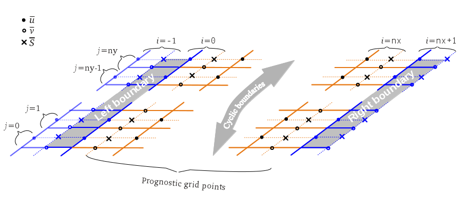
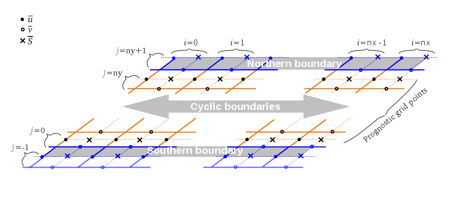
By default, lateral boundary conditions are set to be cyclic in both directions. Alternatively, it is possible to opt for non-cyclic conditions in one direction, i.e., a laminar or turbulent inflow boundary (see Sect. Laminar and turbulent inflow boundary conditions) and an open outflow boundary on the opposite site (see Sect. Open outflow boundary conditions). The boundary conditions for the other direction have to remain cyclic.

In order to prevent gravity waves from being reflected at the top boundary, a sponge layer (Rayleigh damping) can be applied to all prognostic variables in the upper part of the model domain (Klemp and Lilly, 1978). Such a sponge layer should be applied only within the free atmosphere, where no turbulence is present.

The model is initialized by horizontally homogeneous vertical profiles of potential temperature, specific humidity (or a passive scalar), and the horizontal wind velocities. The latter can be also provided from a 1-D precursor run (see Sect.1-D model for precursor runs). Uniformly distributed random perturbations with a user-defined amplitude can be imposed to the fields of the horizontal velocities components to initiate turbulence.

Laminar and turbulent inflow boundary conditions

In case of laminar inflow, Dirichlet boundary conditions are used for all quantities, except for the SGS-TKE e and perturbation pressure π^∗ for which Neumann boundary conditions are used. Vertical profiles, as taken for the initialization of the simulation, are used for the Dirichlet boundary conditions. In order to allow for a fast turbulence development, random perturbations can be imposed on the velocity fields within a certain area behind the inflow boundary (inlet). These perturbations may persist for the entire simulation. For the purpose of preventing gravity waves from being reflected at the inlet, a relaxation area can be defined after Davies (1976). So far, it was found to be sufficient to implement this method for temperature only. This is hence realized by an additional term in the prognostic equation for θ (see third equation in Sect. governing equation):

$\begin{align*} \frac{\partial \theta}{\partial t} = \ldots - C_{\text{relax}} \left(\theta - \theta_{\text{inlet}}\,\right). \end{align*}$

Here, θ_inlet is the stationary inflow profile of θ, and C_relax is a relaxation coefficient, depending on the distance d from the inlet, viz.

$\begin{align*} &C_{\text{relax}}(d) = \begin{cases} F_{\text{inlet}} \cdot \sin^2 \left(\frac{\pi}{2} \frac{D - d}{D} \right) & \text{for~} d < D,\\ 0 & \text{for~} d \ge D,\\ \end{cases} \end{align*}$

with D being the length of the relaxation region and F_inlet being a damping factor.

Turbulence recycling

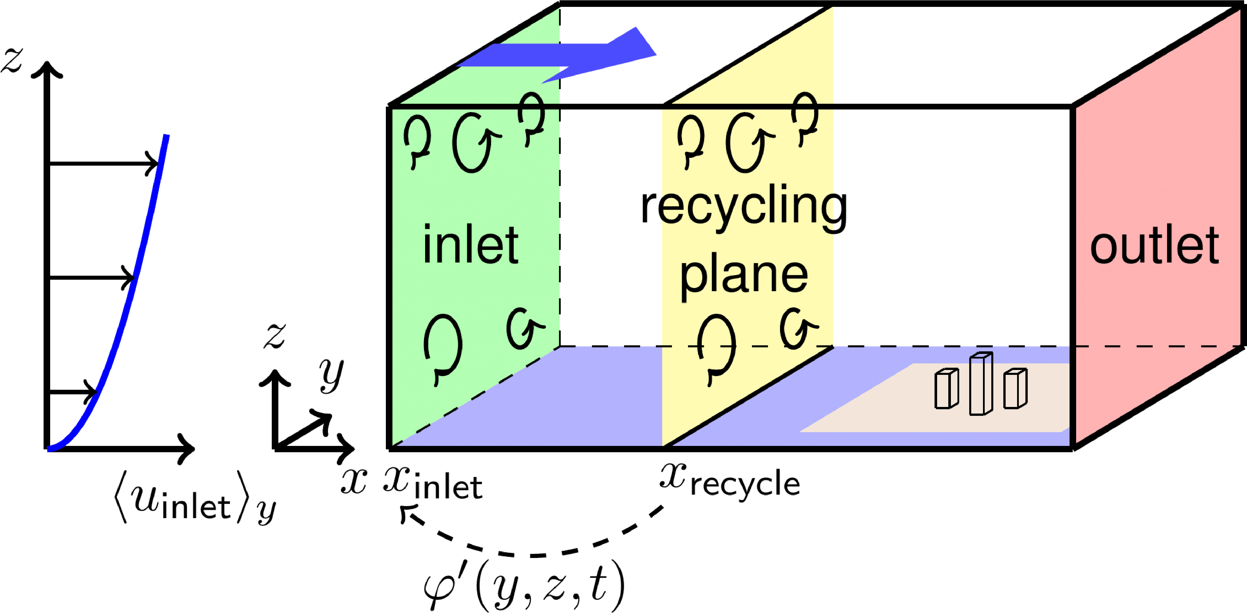
If non-cyclic horizontal boundary conditions are used, PALM offers the possibility of generating time-dependent turbulent inflow data by using a turbulence recycling method. The method follows the one described by Lund et al. (1998), with the modifications introduced by Kataoka and Mizuno (2002). Figure 3 gives an overview of the recycling method used in PALM.

Figure 2: Schematic figure of the turbulence recycling method used for generation of turbulent inflow. The configuration represents exemplary conditions with a built-up analysis area (brown surface) and an open water recycling area (blue surface). The blue arrow indicates the flow direction.

The turbulent signal φ^'(y, z, t) is taken from a recycling plane which is located at a fixed distance x_recycle from the inlet:

$\begin{align*} & \varphi^{\prime}(y, z, t) = \varphi(x_{\text{recycle}},y, z, t) - \langle \varphi\rangle_y(z, t), \end{align*}$

where <φ>_y(z, t) is the line average of a prognostic variable φ ∈ {u, v, w, θ, e} along y at x = x_recycle. φ^'(y, z, t) is then added to the mean inflow profile <φ_inflow>_y(z) at x_inlet after each time step:

$\begin{align*} & \varphi_{\text{inlet}}(y, z, t) = \langle \varphi_{\text{inlet}}\rangle_y(z) + \phi(z) \varphi^{\prime}(y, z, t), \end{align*}$

with the inflow damping function Φ(z), which has a value of 1 below the initial boundary layer height, and which is linearly damped to 0 above, in order to inhibit growth of the boundary layer depth. <φ_inlet>_y(z) is constant in time and either calculated from the results of the precursor run or prescribed by the user. The distance x_recycle has to be chosen much larger than the integral length scale of the respective turbulent flow. Otherwise, the same turbulent structures could be recycled repeatedly, so that the turbulence spectrum is illegally modified. It is thus recommended to use a precursor run for generating the initial turbulence field of the main run. The precursor run can have a comparatively small domain along the horizontal directions. In that case the domain of the main run is filled by cyclic repetition of the precursor run data. Note that the turbulence recycling has not been adapted for humidity and passive scalars so far.

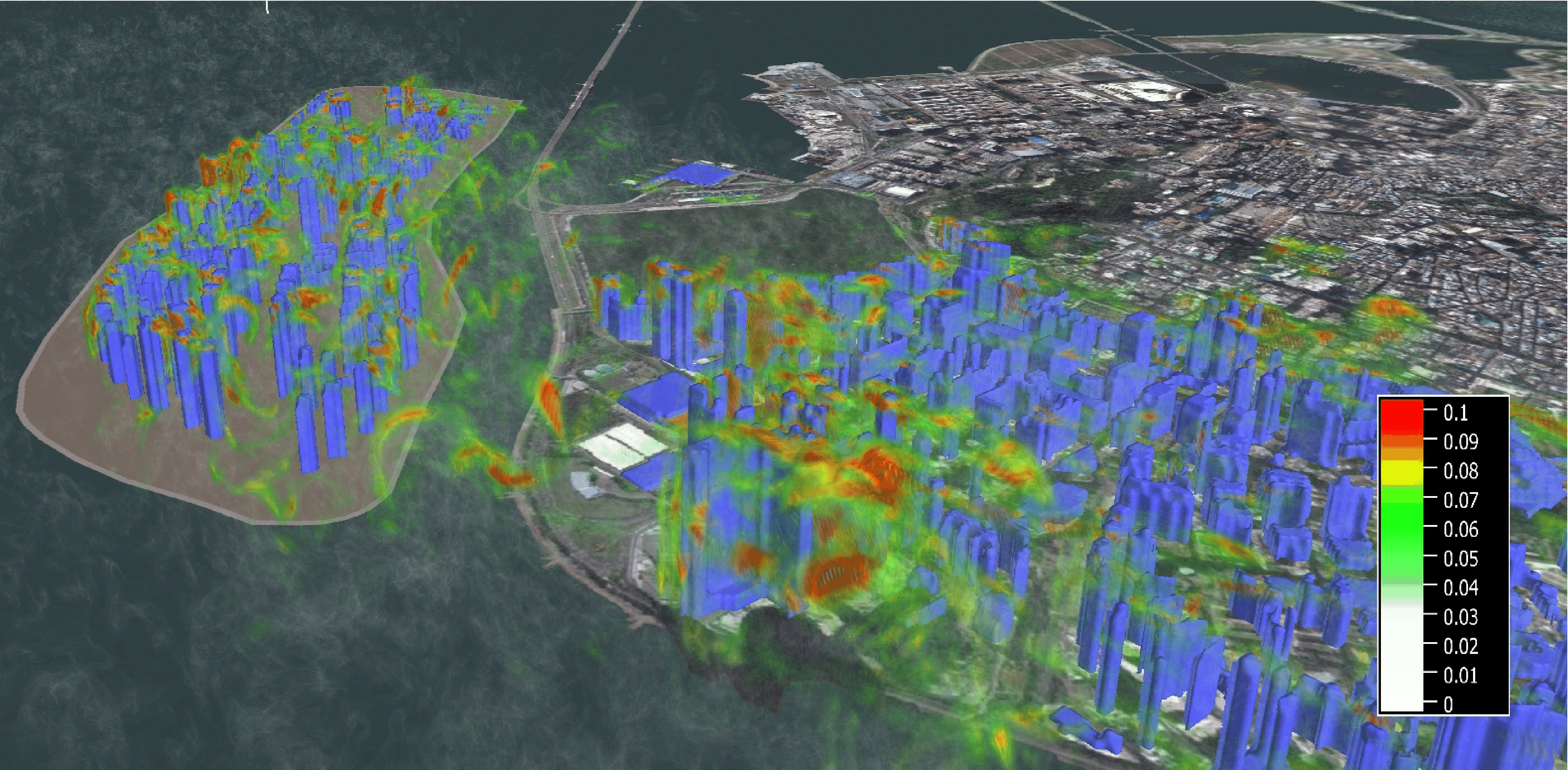
Turbulence recycling is frequently used for simulations with urban topography. In such a case, topography elements should be placed sufficiently downstream of x_recycle to prevent effects on the turbulence at the inlet.

Open outflow boundary conditions

Topography

References

Holtslag AAM, Bruin HARD. 1988. Applied modelling of the night-time surface energy balance over land. J. Appl. Meteorol. 27: 689–704.

Panofsky HA, Dutton JA. 1984. Atmospheric Turbulence, Models and Methods for Engineering Applications. John Wiley & Sons. New York.

Paulson CA 1970. The mathematical representation of wind speed and temperature profiles in the unstable atmospheric surface layer. J. Appl. Meteorol. 9: 857–861.

Klemp JB, Lilly DK. 1978. Numerical simulation of hydrostatic mountain waves. J. Atmos. Sci. 35: 78–107.

Davies HC. 1976. A lateral boundary formulation for multi-level prediction models. Q. J. Roy. Meteor. Soc. 102: 405–418.

Lund TS, Wu X, Squires KD. 1998. Generation of turbulent inflow data for spatially-developing boundary layer simulations. J. Comput. Phys. 140: 233–258.

Kataoka H, Mizuno M. 2002. Numerical flow computation around aerolastic 3d square cylinder using inflow turbulence. Wind Struct. 5: 379–392.

Attachments (6)

03.png (465.4 KB) - added by Giersch 9 years ago. Turbulence recycling method
04.png (91.3 KB) - added by Giersch 9 years ago. Sketch of the 2.5-D implementation of topography
05.png (5.0 MB) - added by Giersch 9 years ago. Snapshot of turbulence structures induced by a densely built-up artificial island of the coast of Macau, China
grid_lr.png (89.4 KB) - added by Giersch 9 years ago. Grid structure at the lateral boundaries with non-cyclic lateral boundary conditions along the left-right direction
grid_ns.png (74.7 KB) - added by Giersch 9 years ago. Figure 2: Grid structure of the lateral boundaries with non-cyclic lateral boundary conditions along the north-south direction.
mask_method.png (19.6 KB) - added by suehring 8 years ago.

Download in other formats:

Plain Text