Overview

This page is part of the Indoor climate and energy demand model (ICM) documentation.
It contains fundamental principles and the equations used in the model.
For an Overview of all ICM-related pages, see the Indoor model main page.

PALM offers an embedded indoor model. It takes account of the heat transfer through exterior walls, the shortwave solar gains and the heat transport by ventilation. It also considers internal heat gains, the energy demand for heating and cooling of the building. According to the building energy concept, the energy demand results in an (anthropogenic) waste heat, that is directly transferred to the urban environment.

The ICM has to work in tandem with the Urban surface model (USM) and the indoor model is only available if the USM activated. The used parameters for ICM can be find in the building database in the USM.

All symbols and parameter are in table 1.

Geometrical calculations

For the initialization stage, it is important to calculate the vital main geometrics of the domain. Every grid point indicates if there is a building and what type. Furthermore, they store the presents of horizontal or vertical façade elements placed at the grid point. With the knowledge of these parameters from every grid point it is possible to assemble the complete façade of a building as sum of single horizontal and vertical façades elements.

A single façade element is the area of one grid point.

The total area of the façade is the sum of all single areas where a façade is located.

To represent the opaque wall and transparent window areas in buildings, a window fraction for horizontal and vertical surfaces gives the ratio of window to wall at a single façade element. The sum of each elemental ratio gives the ratio of the entire building. The ratio of the window area x_win,hv is a parameter of the USM.

The total volume of a building is the sum of all elemental grid volumes where a building is located.

To take respect of an non rectangular building a virtual façade area specific indoor volume shown in figure 1, created.

Figure 1. Scheme of virtual facade area soecific indoor volume

To calculate all façade elements of the whole façade, it is necessary to create an indoor surface area per façade element.

The complete ground surface of a building involves every storey gets a ground surface. To represent this, a net floor area is calculated. The height of the storey h_storey is a parameter of USM.

The effective mass of a specific area takes respect of surfaces like ceilings, walls and furnishing.

The ratio of effective area Λ_𝐴𝑇 and the dynamic parameter of specific effective surface 𝑎 are parameters of the USM.

Model scheme

The ICM is part of the DIN EN ISO 13790:2008 with simplfified dynamic hour-based procedure.

The ICM is based on an analytical solution of Fourier’s law considering a resistance model with five resistances R [K/W] and one heat capacity C [J/K] as seen in figure 2.

Figure 2. Scheme of the 5R1C indoor model

The solution is based on a Crank-Nicolson scheme for a one-hour time step. Since the calculations are based on heat transfer coefficients, H [W/K] all figures and equations are based on heat transfer coefficients. This is the reciprocal value of R and takes short wave, long wave, convective and conductive heat transfer and heat transport (by air) into account.

Resistance and capacity calculations

From a numerical perspective, this network consists of five reciprocal resistances H and one heat storage capacity C:
H_v is the heat transport by ventilation between surface-near exterior air from DIN EN ISO 13789. ϑ_n and indoor air ϑ_i. It is calculated with,

The volumetric heat capacity of air ρ_air⋅c_p is assumed as 0.33⋅W h K⁻¹ m^-3. The schedule on-time Z_sched , the airflow time of occupancy c_ACH,high , the airflow time of no occupancy c_ACH,low and the efficiency of heat recovery in the ventilation η_v are parameters of the USM.

H_t,is is the connective heat transfer between indoor air ϑ_i and interior surface ϑ_s considering all room-enclosing surfaces.

H_t,es is the heat transfer through windows between exterior air ϑ_e and interior surfaces ϑ_s .

h_es is the specific heat transfer coefficient through windows between exterior air and interior surface. Because of the model structure the specific heat transfer coefficient between indoor air and interior surface is removed. H_t,ms is the conductive heat transfer between interior surface ϑ_s and interior mass node ϑ_m .

H_t,wm is the conductive heat transfer between wall ϑ_w and interior mass node ϑ_m .

With H_t,wall as heat transfer of opaque components.

The thickness 𝑑_{𝑙𝑎𝑦𝑒𝑟4} and the thermal heat conductivity 𝜆_{𝑙𝑎𝑦𝑒𝑟4} of the fourth layer are a parameter of USM.
H_t,1 , H_t,2 and H_t,3 are auxiliary variables for calculation of the heat transport.

C_m is the internal heat capacity.

Thermal load and temperature calculations

The internal air load is calculated with the internal heat gains with respect of occupancy of the building. The schedule is a parameter of the USM.

Φ_sol is the heat load from shortwave radiation through all windows in respect of automatic window shutters. At a value of 300 W m^-2 shortwave radiation, the automatic window shutters are set as on. With activated the shutters the shading factor f_c of the sun protection take effect. The shading factor f_c and the g-value g_win are parameters of the USM based on DIN 4108-2.

Φ_st is the mass specific heat load (without thermal mass).

Φ_m is the mass specific heat load for internal and external heat sources of the inner node.

ϑ_ind,wall is the weighted temperature of innermost wall layer.

The fractions for wall/vegetation 𝑥_{𝑤𝑎𝑙𝑙,𝑣𝑒𝑔} and window 𝑥_{𝑤𝑖𝑛,ℎ𝑣} are parameters imported from Land surface model (LSM). The temperatures for wall/vegetation 𝜗_{𝑤𝑎𝑙𝑙,𝑣𝑒𝑔} and for windows 𝜗_𝑤𝑖𝑛 are parameters imported from USM.
Φ_{𝑚,𝑡𝑜𝑡} is the of total mass specific thermal load, internal and external.

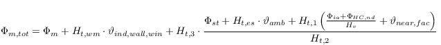
The ambient temperature 𝜗_𝑎𝑚𝑏 is the undisturbed outside temperature and an input of PALM Model. The near façade temperature 𝜗_{𝑛𝑒𝑎𝑟,𝑓𝑎𝑐} is the outside air temperature 10 cm away from the façade and an input of the Land surface model (LSM).

ϑ_m,t is the (fictive) component temperature at actual time step.

ϑ_m,t,prev is the (fictive) component temperature at previous time step.
ϑ_s is the surface temperature at actual time step.

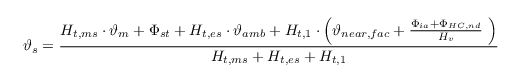
ϑ_air is the indoor air temperature.

ϑ_op is the operative temperature. The operative temperature is a weighted average of the indoor air temperature and mean radiation temperature.

Heating and Cooling Demand

The heating and cooling demand Φ_HC,nd is disposed in 5 different stages as shown in figure 3.

Figure 3. Scheme for heating and coolimg demand. Stage 2 is preparation for stage 3

Stage 1: No heating or cooling necessary, because room temperature ϑ_air is between the set comfort temperatures when heating ϑ_heat,set or cooling ϑ_cool,set is needed. In this case the demand is:

The calculated indoor air temperature is described as ϑ_air,0 .

Stage 2: If the room temperature is outside the comfort threshold, heating or cooling are needed. Then the heating/cooling power is calculated with 10 W m^-2 as Φ_HC,10 .

The indoor air temperature ϑ_air,10 is calculated again with Φ_HC,10 .
ϑ_air,set is the intended air temperature depended of heating ϑ_h,set and cooling ϑ_c,set .

The intended air temperatures for heating ϑ_(h,set) and for cooling ϑ_c,set are parameters of USM.
To estimate the needed amount of heating/ cooling, the unlimited heating/cooling demand Φ_HC,nd,un is calculated without the consideration of the maximum thermal capacity.

Stage 3: Checking if the unlimited heating/cooling demand Φ_HC,nd,un lower as the maximal heating Φ_heat,max or cooling Φ_cool,max power, than is the heat/cooling demand Φ_HC,nd equal the unlimited heating/cooling demand Φ_HC,nd,un .

Stage 4: If the unlimited heating or cooling demand is higher than the maximal heating Φ_heat,max or cooling Φ_cool,max power the heating demand is assumed as the maximum heating flux.

And the cooling demand is maximum cooling heat flux.

The maximal heating Φ_heat,max and cooling Φ_cool,max power is calculated with the heat flux q_h,max and q_c,max which are parameters of USM.

In this case, the set indoor temperature is not reachable. It will get higher than the requested indoor temperature in summer (cooling) cases and colder in winter (heating) cases.

Heat fluxes and waste heat

q_wall is the heat flux through the walls.

q_win is the heat flux through windows.

q_waste is the waste heat through walls/windows with respect on heating/cooling demand and the efficiency of heating/cooling technology. c_heat,on and c_cool,on are flags to separate heating and cooling technology. Whilst the possible values for c_heat,on are 0 and 1 the possible values for c_cool,on are 0 and -1 because the Cooling demand Φ_HC,nd is negative, but anthropogenic waste heat q_waste always be positive.

The anthropogenic heat parameter for heating c_(waste,heat) and cooling c_(waste,cool) are parameters of USM.

Table 1. List of symbols and parameters of indoor model