Context Navigation

Turbulence Parameterization

Since r2696, PALM can be operated as a RANS (Reynolds-averaged Navier-Stokes) model. When running PALM as a RANS model, a different turbulence closure is used compared to the LES model where the turbulence kinetic energy (TKE) e is completely parameterized.

Two different turbulence models are available:

which are described below.

PALM is automatically switched into RANS mode if one of the above listed turbulence parameterizations is selected. The turbulence parameterization can be selected via the namelist parameter turbulence_closure.

Prior to r3545, the namelist parameter rans_mode needs to be set to .TRUE. in addition of selecting one of the turbulence parameterizations if the RANS mode shall be used.

TKE-l model

The TKE-l model calculates the eddy diffusivities via the turbulence kinetic energy e and the mixing length l:

$\begin{align*} K_\mathrm{m} &= c_0 \ l \ \sqrt{e}, \\ K_\mathrm{h} &= \frac{K_\mathrm{m}}{\mathrm{Pr}}, \end{align*}$

where Pr denotes the Prandtl number. The model constant c₀ is set to 0.55 by default, but can be altered via the namelist parameter rans_const_c.

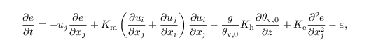
The TKE is calculated using the following prognostic equation:

$\begin{equation*} \frac{\partial{e}}{\partial t} = - u_j\frac{\partial e}{\partial x_j} + K_\mathrm{m} \left( \frac{\partial u_i}{\partial x_j} + \frac{\partial u_j}{\partial x_i} \right) \frac{\partial u_i}{\partial x_j} - \frac{g}{\theta_{\mathrm{v},0}} K_\mathrm{h} \frac{\partial \theta_{\mathrm{v},0}}{\partial z} + K_\mathrm{e} \frac{\partial^2 e}{\partial x_j^2} - \varepsilon, \end{equation*}$

where K_e is defined as

$\begin{align*} K_\mathrm{e} &= \frac{K_\mathrm{m}}{\sigma_e}, \end{align*}$

with σ_e = 1. This can be altered via the namelist parameter rans_const_sigma. The dissipation rate ε of the TKE is calculated via

$\begin{equation*} \varepsilon = c_0^3 \ e \ \frac{\sqrt{e}}{l}. \end{equation*}$

The mixing length is defined using the mixing length l_B according to Blackadar (1962) and the Dyer-Businger function Φ_m

$\begin{align*} l &= \min\left( \frac{l_\mathrm{B}}{\Phi_\mathrm{m}}, l_\mathrm{wall} \right), \\ l_\mathrm{B} &= \dfrac{\kappa z}{1+\frac{\kappa z}{\lambda}}, \\ \lambda &= 2.7 \cdot 10^{-4} |U_g| f, \\ \Phi_\mathrm{m} &= 1+5\frac{z}{L}, \end{align*}$

where κ, f, U_g, L, and z denote the von-Karman constant, the Coriolis parameter, the geostrophic wind, the Obukhov length, and the height, respectively. l_wall defines an upper limit of the mixing length as the distance to the nearest solid surface (wall).

TKE-ε model

The TKE-ε model calculates the eddy diffusivities via the turbulence kinetic energy e and the dissipation rate ε of the TKE:

$\begin{align*} K_\mathrm{m} &= c_0^4 \ \frac{e^2}{\varepsilon}, \\ K_\mathrm{h} &= \frac{K_\mathrm{m}}{\mathrm{Pr}}, \end{align*}$

where Pr denotes the Prandtl number. The model constant c₀ is set to 0.55 by default, but can be altered via the namelist parameter rans_const_c.

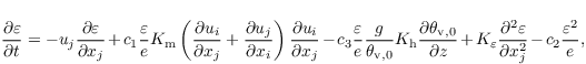
The TKE is calculated using the same prognostic equation as the TKE-l model. The dissipation rate ε is calculated via the following prognostic equation:

$\begin{equation*} \frac{\partial{\varepsilon}}{\partial t} = - u_j\frac{\partial \varepsilon}{\partial x_j} + c_1 \frac{\varepsilon}{e} K_\mathrm{m} \left( \frac{\partial u_i}{\partial x_j} + \frac{\partial u_j}{\partial x_i} \right) \frac{\partial u_i}{\partial x_j} - c_3 \frac{\varepsilon}{e} \frac{g}{\theta_{\mathrm{v},0}} K_\mathrm{h} \frac{\partial \theta_{\mathrm{v},0}}{\partial z} + K_\varepsilon \frac{\partial^2 \varepsilon}{\partial x_j^2} - c_2 \frac{\varepsilon^2}{e}, \end{equation*}$

where K_ε is defined as

$\begin{equation*} K_\varepsilon = \frac{K_\mathrm{m}}{\sigma_\varepsilon} \end{equation*}$

with σ_ε = 1.3. This can be altered via the namelist parameter rans_const_sigma. The model constants c₁, c₂, and c₃ are set to 1.44, 1.92, and 1.44, respectively. These values can be altered via the namelist parameter rans_const_c.

Boundary conditions for e, ε, and K_m are

$\begin{align*} e &= \left( \frac{u_*}{c_0} \right)^2, \\ \varepsilon &= \frac{u_*^3}{\kappa z_\mathrm{MO}}, \\ K_\mathrm{m} &= \kappa \ u_* \ z_\mathrm{MO} \ \Phi_\mathrm{m}^{-1}(\frac{z_\mathrm{MO}}{L}), \end{align*}$

where u_* denote the friction velocity. Note that Φ_m is only used for horizontal boundaries.

Last modified 3 years ago Last modified on Feb 23, 2021 3:22:31 PM

Download in other formats:

Plain Text