Home

Context Navigation

Version 8 (modified by maronga, 9 years ago) (diff)
--

Land surface model

Overview

Since r1551 a full land surface model (LSM) is available in PALM. It consists of a four layer soil model, predicting soil temperature and moisture content, and a solver for the energy balance of the skin surface layer. Moreover, a liquid water reservoir accounts for the presence of liquid water on plants and soil due to precipitation. The implementation is based on the ECMWF-IFS land surface parametrization (H-TESSEL) and its adaptation in the DALES model (Heus et al. 2010).

Note that the use of the LSM requires using a radiation model to provide radiative fluxes at the surface.

Energy balance solver

The energy balance of the Earth's surface reads

$\begin{equation*} C_0 \dfrac{dT_0}{dt} = R_\mathrm{n} - H - LE - G \end{equation*}$

where C₀ and T₀ are the heat capacity and radiative temperature of the surface skin layer, respectively. R_n, H, LE, and G are the net radiation, sensible heat flux, latent heat flux, and ground (soil) heat flux at the surface, respectively. H is calculated as

$\begin{equation*} H = - \rho\ c_\mathrm{p}\ \dfrac{1}{r_\mathrm{a}} ( \theta_1 - \theta_0 ) \end{equation*}$

where ρ is the density of the air, c_p = 1005 J kg^-1 K^-1$ is the specific heat at constant pressure, r_a is the aerodynamic resistance, and θ₀ and θ₁ are the potential temperature at the surface and at the first grid level above the surface, respectively. r_a is calculated via Monin-Obukhov similarity theory, based on roughness lengths for heat and momentum and the assumption of a constant flux layer between the surface and the first grid level.

G is parametrized as (Duynkerke 1999)

$\begin{equation*} G = \Lambda ( T_0 - T_{\mathrm{soil},1} ) \end{equation*}$

with Λ being the heat conductivity between skin layer and the soil, and T_soil,1 being the temperature of the uppermost soil layer. The latent heat flux is calculated as

$\begin{equation*} LE = - \rho\ l_\mathrm{v}\ \dfrac{1}{r_\mathrm{a} + r_\mathrm{s}} ( q_{\mathrm{v},1} - q_{\mathrm{v,sat}}(T_0) )\;. \end{equation*}$

Here, l_v = 2.5 * 10⁶ J kg^-1 is the latent heat of vaporisation, r_s is the surface resistance, q_v,1 is the specific humidity at first grid level, and q_v,sat is the saturation specific humidity at temperature T₀.

All equations above are solved locally for each surface element of the LES grid. Each element can consist of both patches of bare soil, vegetation, and a liquid water reservoir, which is the interception water stored on plants and soil from precipitation. Therefore, an additional equation is solved for the liquid water reservoir. LE is then calculated for each of the three components (bare soil, vegetation, liquid water). The resistances are calculated following Jarvis (1976).

C₀ is set to zero, the energy balance is solved implicitly by linearising q_v,sat.

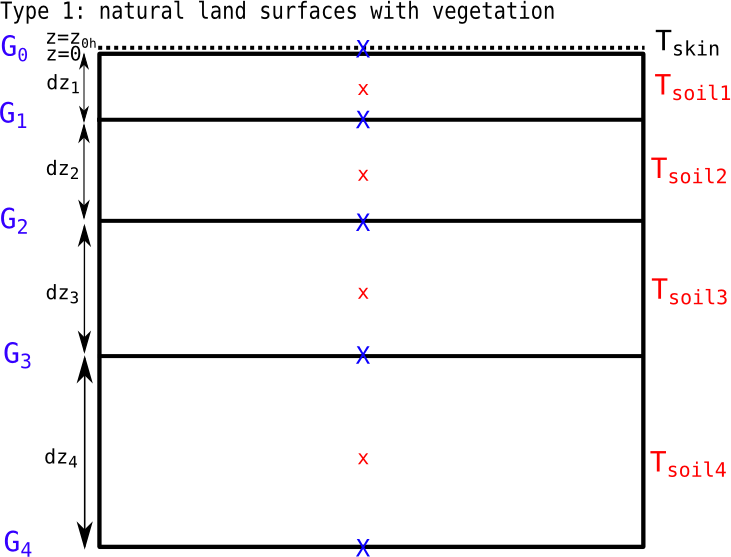
Soil model

Technical details

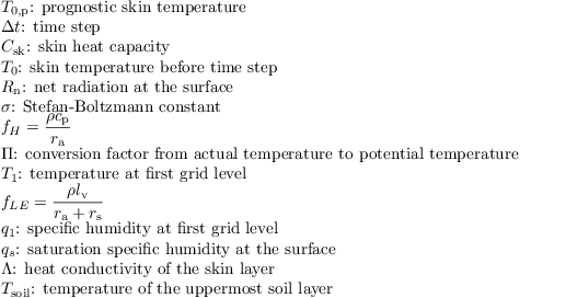
The discretized and linearized energy budget equation in PALM reads

$\begin{equation*} T_\mathrm{0,p} = \dfrac{A \Delta t + C_\mathrm{sk} T_0}{C_\mathrm{sk} + B \Delta t} \end{equation*}$

with

$\begin{equation*} A = R_\mathrm{n} + 3 \sigma T_0^4 + \dfrac{f_H}{\Pi} T_1 + f_{LE} \left( q_1 - q_s + \dfrac{d q_s}{d T} T_0 \right) + \Lambda T_\mathrm{soil} \end{equation*}$

and

$\begin{equation*} B = \Lambda + f_{LE} \dfrac{d q_s}{d T} + \dfrac{f_H}{\Pi} + 4 \sigma T_0^3 \end{equation*}$

with (in order of occurence):

$$T_\mathrm{0,p}$: prognostic skin temperature\\ $\Delta t$: time step\\ $C_\mathrm{sk}$: skin heat capacity\\ $T_\mathrm{0}$: skin temperature before time step\\ $R_\mathrm{n}$: net radiation at the surface\\ $\sigma$: Stefan-Boltzmann constant\\ $f_{H} = \dfrac{\rho c_\mathrm{p}}{r_\mathrm{a}}$\\ $\Pi$: conversion factor from actual temperature to potential temperature\\ $T_1$: temperature at first grid level\\ $f_{LE} = \dfrac{\rho l_\mathrm{v}}{r_\mathrm{a} + r_\mathrm{s}}$\\ $q_1$: specific humidity at first grid level\\ $q_s$: saturation specific humidity at the surface\\ $\Lambda$: heat conductivity of the skin layer\\ $T_\mathrm{soil}$: temperature of the uppermost soil layer$

Usage

References

Attachments (2)

2015_LSM.pdf (2.8 MB) - added by maronga 10 years ago. LSM introduction
wall_concept_type1.png (34.1 KB) - added by maronga 8 years ago. soil model (vegetation)

Download in other formats:

Plain Text