
| Version 62 (modified by westbrink, 5 years ago) (diff) |
|---|
Land surface model
This page is part of the Land Surface Model (LSM) documentation.
It describes the physical and numerical realization of the LSM.
Please also see the namelist parameters.
Overview
Since r1551 a full land surface model (LSM) is available in PALM (see land_surface_model_mod.f90). It consists of a multi layer soil model, predicting soil temperature and moisture content, and a solver for the energy balance, predicting the temperature of the surface or the skin layer (depending on land use classification). Moreover, a liquid water reservoir accounts for the presence of liquid water on plants, pavement, and bare soil due to precipitation. The implementation is based on the ECMWF-IFS land surface parametrization (H-TESSEL) and its adaptation in the DALES model (Heus et al. 2010).
Note that the use of the LSM requires using some kind of radiation model to provide radiative fluxes at the surface.
Energy balance solver
The energy balance of the Earth's surface reads

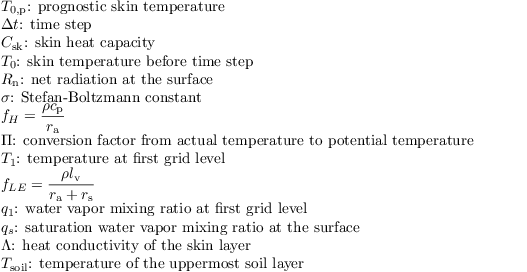
where C0 and T0 are the heat capacity and radiative temperature of the surface skin layer, respectively. Note that C0 is usually zero as it is assumed that the skin layer does not have a heat capacity (see also below). Rn, H, LE, and G are the net radiation, sensible heat flux, latent heat flux, and ground (soil) heat flux at the surface, respectively.
Parameterization of H
H is calculated as

where ρ is the density of the air, cp = 1005 J kg-1 K-1 is the specific heat at constant pressure, ra is the aerodynamic resistance, and θ0 and θ1 are the potential temperature at the surface and at the first grid level above the surface, respectively. ra is calculated via Monin-Obukhov similarity theory, based on roughness lengths for heat and momentum and the assumption of a constant flux layer between the surface and the first grid level:

where u* and θ* are the friction velocity and the characteristic temperature scale according to Monin-Obukhov similarity scaling (these are calculated in surface_layer_fluxes_mod.f90).
Parameterization of G
G is parametrized as (see Duynkerke 1999)

with Λ being the total thermal conductivity between skin layer and the uppermost soil layer, and Tsoil,1 being the temperature of the uppermost soil layer. Λ is calculated as a combination of the conductivity between the canopy and the soil-top (constant value) and the conductivity of the top half of the uppermost soil layer:

When no skin layer is used (i.e. in case of bare soil and pavements), Λ reduces to the heat conductivity of the uppermost soil layer (divided by the layer depth). In that case, it is assumed that the soil temperature is constant within the uppermost 1/4 of the top soil layer and equals the radiative temperature. C0 is then set to a non-zero value according to the material properties.
Parameterization of LE
The latent heat flux is calculated as

Here, lv = 2.5 * 106 J kg-1 is the latent heat of vaporisation, rs is the surface resistance, qv,1 is the water vapor mixing ratio at first grid level, and qv,sat is the water vapor mixing ratio at temperature T0.
All equations above are solved locally for each surface element of the LES grid. Each element for the surface type 'vegetation' can consist of patches of bare soil, vegetation, and a liquid water reservoir, which is the interception water stored on plants and soil from precipitation. Therefore, an additional equation is solved for the liquid water reservoir. A liquid water reservoir is also available when the surface type is set to 'pavement'. LE is then calculated for each of the three components (bare soil, vegetation, liquid water). The resistances are calculated separately for bare soil and vegetation following Jarvis (1976). The canopy resistance is calculated as

with
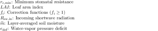
The correction functions read

which accounts for the reaction of plants to shortwave radiation (opening/closing stomata),

where gD is a correction factor (for high vegetation only, otherwise zero). Moreover, the reaction of plants to water availability in the soil is considered:

where

and

where

and N is the number of soil layers.
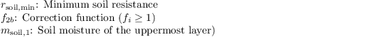
The bare soil resistance is given by

with
The total evapotranspiration is then calculated as

where cveg, and cliq is the surface fraction covered with vegetation and liquid water, respectively.
Prognostic equation for the liquid water reservoir
The prognostic equation for the liquid water stored on plants and bare soil mliq reads

The maximum amount of water that can be stored on plants is calculated via

where m,liq,ref, = 0.2 mm is the reference liquid water column on a single leaf or bare soil. Exceeding liquid water is directly removed from the surface and infiltrated in the underlying soil. For positive values of LEliq, liquid water is evaporating from the surface, while negative values indicate precipitation (rain, dew). The values of c,liq, are calculated either as the ratio

for vegetation (following the HTESSEL scheme, Viterbo & Beljaars, 1995) and
following Masson (2000).
Soil model
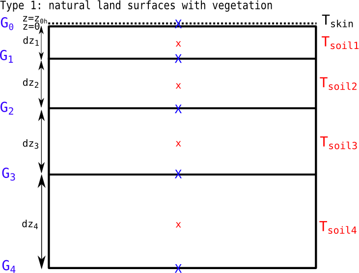
The soil model consists of prognostic equations for the soil temperature and the volumetric soil moisture which are solved for multiple layers. The soil model only takes into account vertical transport within the soil and no ice phase is considered. By default, the soil model consists of eight layers (see Fig. 12 below), in which the vertical heat and water transport is modelled using the Fourier law of diffusion and Richards' equation, respectively. Also, root fractions can be assigned to each soil layer to account for the explicit water withdrawal of plants used for transpiration from the respective soil layer.
")
Figure 12: Default layer distribution in the soil model.
Soil heat transport
The prognostic equation for soil temperature reads

with

The heat conductivity is calculated as

with

The heat conductivity of saturated soil is given by

with

The Kersten number is calculated as
![\begin{equation*}
Ke = \log_{10} \left[max\left(0.1, \dfrac{m_\mathrm{soil}}{m_\mathrm{sat}}\right) \right] + 1
\end{equation*}](/trac/tracmath/e77050c1b4636f38bc44df22df92578fe40c737a.png)
Soil moisture transport
The prognostic equation for volumetric soil moisture reads

with

The hydraulic diffusion coefficient is calculated after Clapp and Hornberger (1978) as

with

The hydraulic conductivity is calculated either after Van Genuchten (1980) (as in H-TESSEL):
![\begin{equation*}
\gamma = \gamma_\mathrm{sat} \dfrac{\left[(1 + (\alpha h)^n)^{1 - 1/n} - (\alpha h)^{n-1}\right]^2}{(1+ (\alpha h)^n)^{(1 - 1/n)(l + 2)}}
\end{equation*}](/trac/tracmath/5b600b1408ec0ddcff47d3193cf9bc73e809981f.png)
where
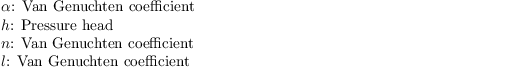
and

Root extraction
The root extraction of water from the respective soil layer Sm is calculated as follows:

where mtotal is the total water content of the soil and Rfr is the root fraction in soil layer k. Only those layer are summed up which have a soil moisture above wilting point (plants do not extract water from such layers). The root profiles must prescribed in such a way that

The root extraction is then given by

Here, dzs(k) is the thickness of layer k. Again, only layers where the soil moisture is above its value at wilting point are used for root extraction (which is zero otherwise).
Boundary conditions
Neumann boundary conditions are used for the transport of heat and moisture at the upper boundary (surface). The values are given by the energy balance in terms of G for heat and LEsoil, for moisture. At the bottom boundary a deep soil temperature is prescribed (Dirichlet conditions), whereas two options are available for soil moisture. The underlying surface can be set to either bedrock (no moisture flux at the bottom, water conserving) or to open bottom (implies non-conservation of water).
For more details, see also Viterbo et al. (1995) and Balsamo et al. (2009).
Exception: water surfaces
When prescribing grid points with water surface (i.e. surface_type = 'water'), the energy balance is solved as for land surface without evaporation from vegetation canopy and bare soil. Moreover, the water temperature is constant in time and is derived from the value of pt_surface at model start. In order to obtain realistic results, it is required to set a zero heat capacity for the ocean skin layer (e.g. c_surface = 0.0).
A special feature of the treatment of water surfaces is the treatment of surface roughness chances due to water waves. The roughness lengths for momentum, heat, and moisture (z0, z0,h, and z0,q respectively) are hence calculated after Beljaars (1994) at each grid point as:

Here, ν is the molecular viscosity, and αCh = 0.018 is the Charnock constant taken from the ECMWF-IFS model.
Please note that this parameterization was developed for large-scale models where waves are a pure subgrid-scale phenomenon. When using large-eddy simulations, however, this might no longer be the case. It has not been studied whether this parameterization is appropriate in such cases and should only be used with caution.
Exception: pavement
It is possible to account for urban land surfaces such as roads by adding a pavement layer to the soil model. This is realized by setting the parameter surface_type = 'pavement'. The pavement is steered via a depth (pave_depth), a heat capacity (pave_heat_capacity), and a heat conductivity (pave_heat_conductivity). The pavement then replaces the upper soil layers up to a depth of pave_depth. In case that pave_depth is between two soil layers, the respective heat conductivity and heat capacities are linearly interpolated between the soil value and the pavement value to the respective grid point.
Note that the pavement layer must be at least have the same depth as the uppermost soil layer. If the prescribed pavement depth is too small, it is automatically set to this minimum depth.
The pavement is able to hold a maximum liquid water column of 1 mm from precipitation, which can also evaporate. The soil below the pavement is assumed to be completely dry.
Technical details
The discretized and linearized energy budget equation in PALM reads

with

and

with (in order of occurence):
Time stepping is the same as in the atmospheric part of the model (default: 3rd-order Runge-Kutta).
Note that for Csk = 0, the prognostic equation for T0,p reduces to a diagnostic equation:

Job preparation
The lsm is activated by specifying a &land_surface_parameters namelist in the _p3d file, e.g.:
 &land_surface_parameters
          surface_type = 'vegetation',
          vegetation_type = 2,
          soil_type = 3,
          conserve_water_content = .T.,
          c_surface = 0.0,
          dz_soil = 0.01, 0.02, 0.04, 0.07, 0.15, 0.21, 0.72, 1.89,
          root_fraction = 0.1, 0.2, 0.3, 0.2, 0.1, 0.05, 0.05, 0.0,
          soil_temperature = 290.0, 289.0, 288.0, 286.0, 285.0, 285.0, 285.0, 285.0,
          deep_soil_temperature = 280.0,
/
In particular, PALM provides a set of predefined land surface types (parameter vegetation_type) for which typical parameters are used to intialize the model. Moreover, a set of predefined soil types can be chosen (parameter soil_type). You can overwrite the default parameters by explicitly prescribing them in the namelist.
Note that the surface albedo is part of the radiation scheme and is steered via the parameter albedo_type.
A complete list of parameters and a detailed description can be found here.
References
- Beljaars, ACM 1994. The parametrization of surface fluxes in large-scale models under free convection. Q. J. R. Met. Soc. 121: 255–270.
- Balsamo G, Vitebo P, Beljaars A, van den Hurk B, Hirschi M, Betts AK, Scipal K. 2009. A revised hydrology for the ECMWF model: Verification from field site to terrestrial water storage and impact in the integrated forecast system. J. Hydrometeorol. 10: 623–643.
- Clapp RB, Hornberger GM. 1978. Empirical Equations for Some Soil Hydraulic Properties. Water Res. Res. 14: 601-604.
- Duynkerke PG. 1999. Turbulence, radiation and fog in Dutch stable boundary layers. Boundary-Layer Meteorol. 90: 447–477, doi:10.1023/A:1026441904734.
- Heus T, Van Heerwaarden CC, Jonker HJJ, Siebesma AP, Axelsen S, Dries K, Geoffroy O, Moene AF, Pino D, De Roode SR, Vil`a-Guerau de Arellano J. 2010. Formulation of the dutch atmospheric large-eddy simulation (dales) and overview of its applications. Geosci. Model Dev. 3: 415–444.
- Jarvis PG. 1976. The interpretation of the variations in leaf water potential and stomatal conductance found in canopies in the field. Philos. Trans. Roy. Soc. London 273B: 593–610.
- Masson, V. 2000. A physically-based scheme for the urban energy budget in atmospheric models, Boundary-layer Meteorol., 94, 357–397.
- van Genuchten M. 1980. A closed form equation for predicting the hydraulic conductivity of unsaturated soils. Soil Sci. Soc. Amer. J. 44: 892–898.
- Viterbo P, Beljaars ACM. 1995. An Improved Land Surface Parameterization Scheme in the ECMWF Model and Its Validation. J. Climate 8: 2716–2748.
Attachments (2)
-
2015_LSM.pdf
(2.8 MB) -
added by maronga 10 years ago.
LSM introduction
-
wall_concept_type1.png
(34.1 KB) -
added by maronga 8 years ago.
soil model (vegetation)