
| Version 2 (modified by maronga, 9 years ago) (diff) |
|---|
Boundary conditions
Constant flux layer
Following Monin-Obukhov similarity theory (MOST) a constant flux layer can be assumed as boundary condition between the surface and the first grid level where scalars and horizontal velocities are defined (k = 1, zMO = 0.5 Δz). It is then required to provide the roughness lengths for momentum z0 and heat z0,h. Momentum and heat fluxes as well as the horizontal velocity components are calculated using the following framework. The formulation is theoretically only valid for horizontally-averaged quantities. In PALM we assume that MOST can be also applied locally and we therefore calculate local fluxes, velocities, and scaling parameters.
Following MOST, the vertical profile of the horizontal wind velocity

is given in the surface layer by

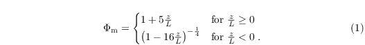
where κ = 0.4 is the Von Kármán constant and Φm is the similarity function for momentum in the formulation of Businger-Dyer (see e.g. Panofsky and Dutton 1984)
Here, L is the Obukhov length, calculated as
(eq:L)![\begin{align}
& \label{eq:L}
L = \frac{\theta_\mathrm{v}(z) u_\ast^2}{\kappa g
\left[\theta_\ast + 0.61 \theta(z) q_\ast + 0.61
q_\mathrm{v}(z) \theta_\ast\right]}\;.
\end{align}](/trac/tracmath/5fb4e0aca386a286e26dec8206fc4668a2776a81.png)
The scaling parameters θ* and q* are defined by MOST as:
(eq:scales)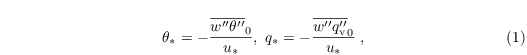
with the friction velocity u* defined as
![\begin{align}
& u_\ast =
\left[\left(\overline{u^{\prime\prime} w^{\prime\prime}}_0\right)^2
+ \left(\overline{v^{\prime\prime} w^{\prime\prime}}_0\right)^2
\right]^{\frac{1}{4}}\;.
\end{align}](/trac/tracmath/055307302220c5342d4f459c29b53e28b47ce90f.png)
In PALM, u* is calculated from uh at zMO by vertical integration over z from z0 to zMO.
From the equations above it is possible to derive a formulation for the horizontal wind components, viz.
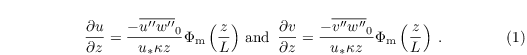
Vertical integration of the above equation over z from z0 to zMO then yields the surface momentum fluxes

The formulations above all require knowledge of the scaling parameters θ* and q*. These are deduced from vertical integration of

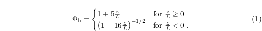
over z from z0,h to zMO. The similarity function Φh is given by
Note that this implementation of MOST in PALM requires the use of data from the previous time step. The following steps are thus carried out in sequential order. First of all, θ* and q* are calculated by integration using the value of zMO/L from the previous time step. Second, the new value of zMO/L is derived using the new values of θ* and q* but using u* from the previous time step. Then, the new values of u*, and subsequently the momentum fluxes are calculated by integration, respectively. At last, the new surface fluxes are derived from θ* and q*, and u*. In the special case, when surface fluxes are prescribed instead of surface temperature and humidity, the first and last steps are omitted and θ* and q* are directly calculated from u* and the surface fluxes.
Attachments (6)
-
03.png
(465.4 KB) -
added by Giersch 9 years ago.
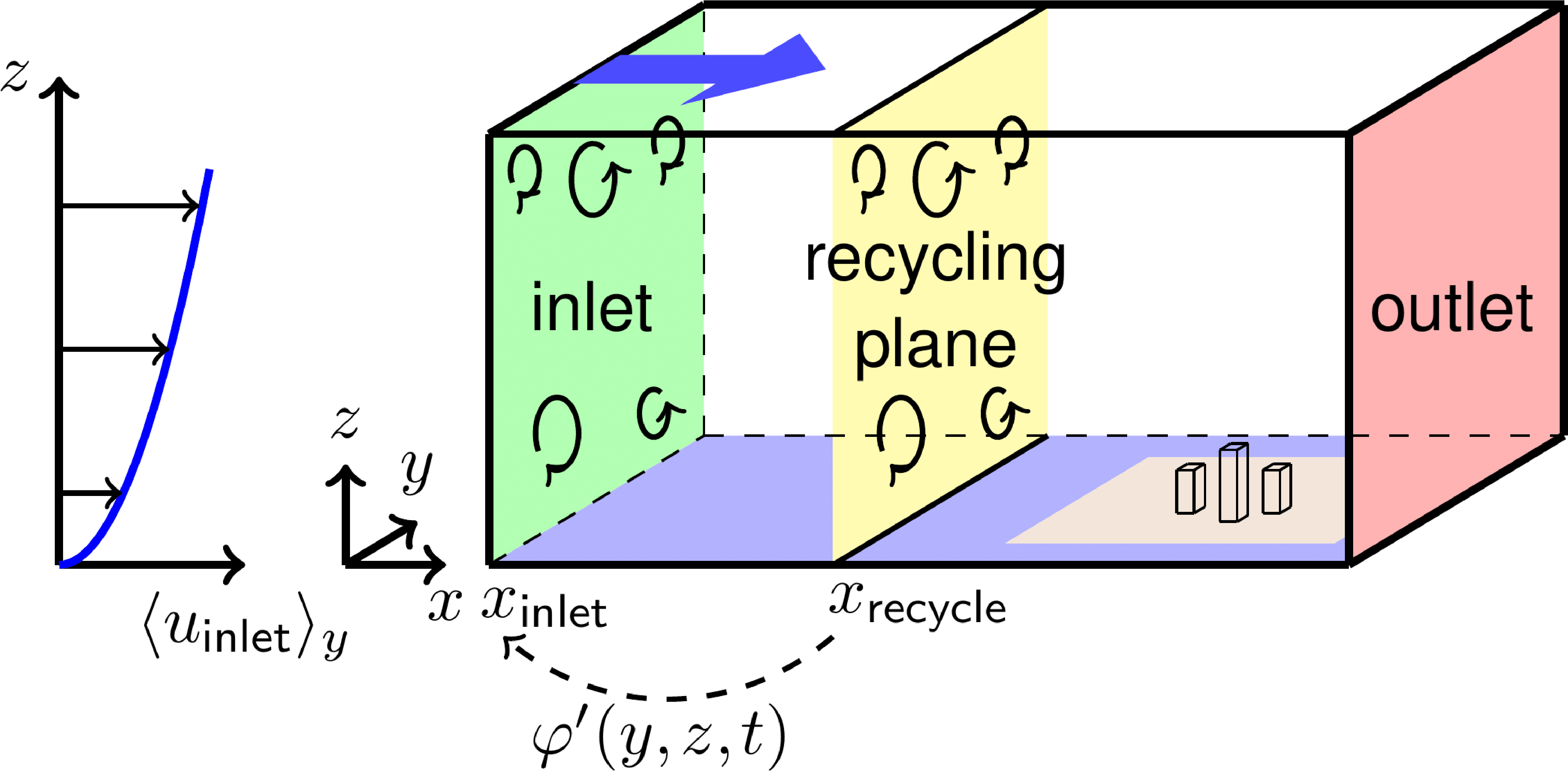
Turbulence recycling method
-
04.png
(91.3 KB) -
added by Giersch 9 years ago.
Sketch of the 2.5-D implementation of topography
-
05.png
(5.0 MB) -
added by Giersch 9 years ago.
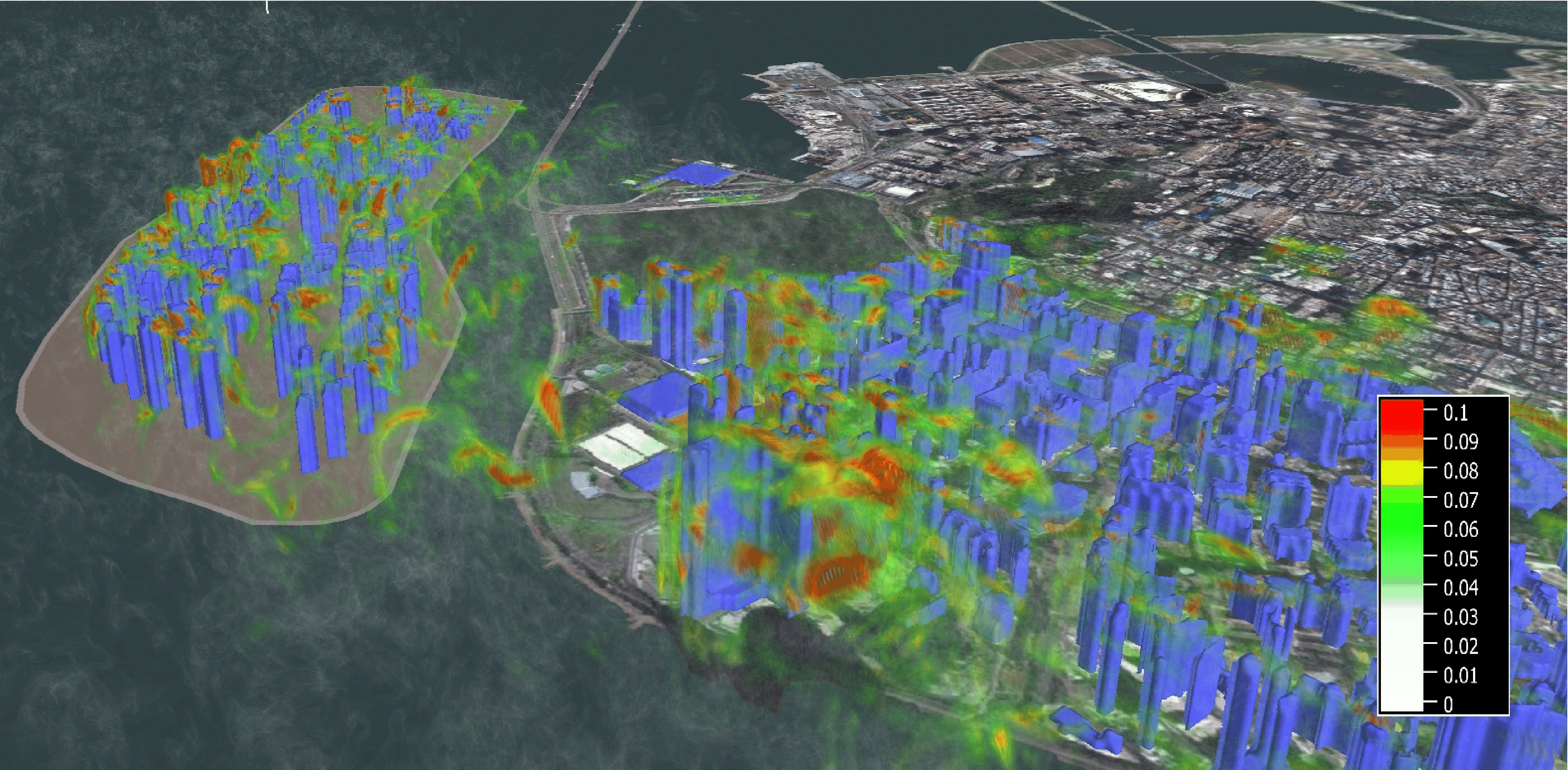
Snapshot of turbulence structures induced by a densely built-up artificial island of the coast of Macau, China
-
grid_lr.png
(89.4 KB) -
added by Giersch 9 years ago.
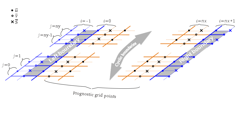
Grid structure at the lateral boundaries with non-cyclic lateral boundary conditions along the left-right direction
-
grid_ns.png
(74.7 KB) -
added by Giersch 9 years ago.
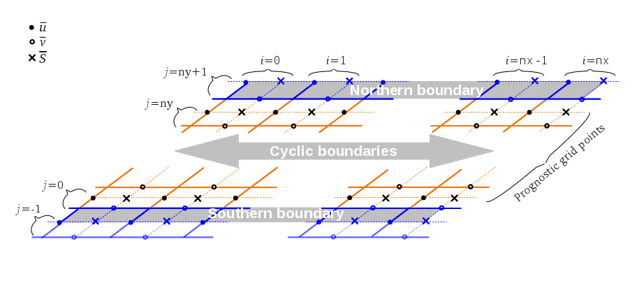
Figure 2: Grid structure of the lateral boundaries with non-cyclic lateral boundary conditions along the north-south direction.
- mask_method.png (19.6 KB) - added by suehring 8 years ago.