
| Version 16 (modified by Giersch, 9 years ago) (diff) |
|---|
Boundary conditions
PALM offers a variety of boundary conditions. Dirichlet or Neumann boundary conditions can be chosen for u, v, θ, qv, and p∗ at the bottom and top of the model. For the horizontal velocity components the choice of Neumann (Dirichlet) boundary conditions yields free-slip (no-slip) conditions. Neumann boundary conditions are also used for the SGS-TKE. Kinematic fluxes of heat and moisture can be prescribed at the surface instead (Neumann conditions) of temperature and humidity (Dirichlet conditions). At the top of the model, Dirichlet boundary conditions can be used with given values of the geostrophic wind. By default, the lowest grid level (k = 0) for the scalar quantities and horizontal velocity components is not staggered vertically and defined at the surface (z = 0). In case of free-slip boundary conditions at the bottom of the model, the lowest grid level is defined below the surface (z = - 0.5 Δz) instead. Vertical velocity is assumed to be zero at the surface and top boundaries, which implies using Neumann conditions for pressure.
Constant flux layer
Basics
Following Monin-Obukhov similarity theory (MOST) a constant flux layer can be assumed as boundary condition between the surface and the first grid level where scalars and horizontal velocities are defined (k = 1, zMO = 0.5 Δz). It is then required to provide the roughness lengths for momentum z0 and heat z0,h. Momentum and heat fluxes as well as the horizontal velocity components are calculated using the following framework. The formulation is theoretically only valid for horizontally-averaged quantities. In PALM we assume that MOST can be also applied locally and we therefore calculate local fluxes, velocities, and scaling parameters.
Following MOST, the vertical profile of the horizontal wind velocity

is given in the surface layer by

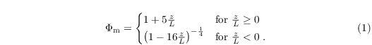
where κ = 0.4 is the Von Kármán constant and Φm is the similarity function for momentum in the formulation of Businger-Dyer (see e.g. Panofsky and Dutton 1984)
Here, L is the Obukhov length, calculated as
![\begin{align}
&
L = \frac{\theta_\mathrm{v}(z) u_\ast^2}{\kappa g
\left[\theta_\ast + 0.61 \theta(z) q_\ast + 0.61
q_\mathrm{v}(z) \theta_\ast\right]}\;.
\end{align}](/trac/tracmath/bafe5aaadfffe15373dea923d2476f266a38f227.png)
The scaling parameters θ* and q* are defined by MOST as:
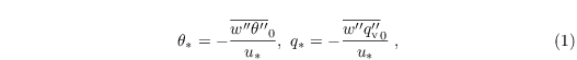
with the friction velocity u* defined as
![\begin{align}
& u_\ast =
\left[\left(\overline{u^{\prime\prime} w^{\prime\prime}}_0\right)^2
+ \left(\overline{v^{\prime\prime} w^{\prime\prime}}_0\right)^2
\right]^{\frac{1}{4}}\;.
\end{align}](/trac/tracmath/055307302220c5342d4f459c29b53e28b47ce90f.png)
In PALM, u* is calculated from uh at zMO by vertical integration over z from z0 to zMO.
From the equations above it is possible to derive a formulation for the horizontal wind components, viz.
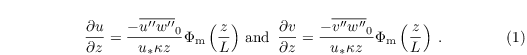
Vertical integration of the above equation over z from z0 to zMO then yields the surface momentum fluxes

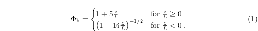
The formulations above all require knowledge of the scaling parameters θ* and q*. These are deduced from vertical integration of

over z from z0,h to zMO. The similarity function Φh is given by
Implementation
Currently, there are three different options to calculate the Obukhov length and the surface fluxes which are steered via the NAMELIST parameter most_method.
Method 1: circular
The traditional implementation in PALM (most_method = 'circular') requires the use of data from the previous time step. The following steps are thus carried out in sequential order. First of all, θ* and q* are calculated by integration using the value of zMO/L from the previous time step. Second, the new value of zMO/L is derived using the new values of θ* and q* but using u* from the previous time step. Then, the new values of u*, and subsequently the momentum fluxes are calculated by integration, respectively. At last, the new surface fluxes are derived from θ* and q*, and u*. In the special case, when surface fluxes are prescribed instead of surface temperature and humidity, the first and last steps are omitted and θ* and q* are directly calculated from u* and the surface fluxes.
In summary, the following actions are performed in sequential order:
- calculate θ* and q*
- calculate uh
- determine Obukhov length
- calculate u*
- derive surface fluxes
Method 2: Newton iteration / lookup table
Alternatively, the Obukhov length can be calculated by solving an implicit equation relating the L to the bulk Richardson number. This can be achieved either by a Newton iteration algorithm (most_method = 'newton') or by using a lookup table (most_method = 'lookup'). Note that the latter is the new default in PALM as it is much faster than the Newton iteration method and the results are more precise compared to the circular method. However, it can only be used when the roughness lengths are homogeneously set on each processor.
Both methods require a different sequential order to derive the surface fluxes:
- calculate uh
- determine Obukhov length (Newton iteration or lookup table)
- calculate u*
- calculate θ* and q*
- derive surface fluxes
Depending on whether Neumann (prescribed fluxes) or Dirichlet boundary conditions are used for temperature and humidity, the bulk Richardson number is related to the Obukhov length via
![\begin{equation*}
Ri_\mathrm{b,Di} = \dfrac{z}{L} \cdot \dfrac{[\phi_\mathrm{H}]}{[\phi_\mathrm{M}]^2} \;\;\;\;\textnormal{(Dirichlet conditions)}
\end{equation*}
\begin{equation*}
Ri_\mathrm{b,Ne} = \dfrac{z}{L} \cdot \dfrac{1}{[\phi_\mathrm{M}]^3} \;\;\;\;\textnormal{(Neumann conditions)}
\end{equation*}](/trac/tracmath/affbeb5be3ff971819f0bd2da16b3c017b2737e4.png)
where
![\begin{equation*}
[\phi_\mathrm{H}] = \log\left(\dfrac{z_\mathrm{MO}}{z_\mathrm{0,h}}\right) - \Phi_\mathrm{H}\left(\dfrac{z_\mathrm{MO}}{L}\right) + \Phi_\mathrm{H}\left(\dfrac{z_\mathrm{0,h}}{L}\right)\;,
\end{equation*}
\begin{equation*}
[\phi_\mathrm{M}] = \log\left(\dfrac{z_\mathrm{MO}}{z_\mathrm{0}}\right) - \Phi_\mathrm{M}\left(\dfrac{z_\mathrm{MO}}{L}\right) + \Phi_\mathrm{M}\left(\dfrac{z_\mathrm{0,h}}{L}\right)\;,
\end{equation*}](/trac/tracmath/b50c08cfdc5202f79c800ecf4d3e820b0f5b7795.png)
are the integrated universal profile stability functions of Φm and Φh (see Paulson 1970, Holtslag and Bruin 1988), and

In case of most_method = 'newton', the above equations are solved for L by Newton iteration, i.e. finding the root of the equation
![\begin{equation*}
f = Ri_\mathrm{b} - \dfrac{z}{L} \cdot \dfrac{[\phi_\mathrm{H}]^x}{[\phi_\mathrm{M}]^y}
\end{equation*}](/trac/tracmath/7cb325324f91240af6df57774f026a77eac1317b.png)
where x and y depend on the chosen boundary conditions (see above). The solution is given by iteration of

with

until L meets a convergence criterion.
If most_method = 'lookup' is used, a table of Rib against zMO/L is created at model start, based on the prescribed values of the roughness lengths. During the model run, Rib is calculated and the respectively value of zMO/L is retrieved from the lookup table and using linear interpolation between the discrete values in the table. In order to speed up this method, the value of Rib from the previous time step is used as initial value. Due to the fact that the lookup table is created at model start, it is essential that the roughness lengths are 1) homogeneous on each processor (limiting this method to homogeneous surface configurations) and should not vary during the simulation (should thus not be used when using dynamic roughness length over water surfaces).
For more details, see surface_layer_fluxes.f90.
References
- Holtslag AAM, Bruin HARD. 1988. Applied modelling of the night-time surface energy balance over land. J. Appl. Meteorol., 27, 689–704.
- Panofsky HA, Dutton JA. 1984. Atmospheric Turbulence, Models and Methods for Engineering Applications, John Wiley & Sons, New York.
- Paulson CA 1970. The mathematical representation of wind speed and temperature profiles in the unstable atmospheric surface layer. J. Appl. Meteorol., 9, 857–861.
Attachments (6)
-
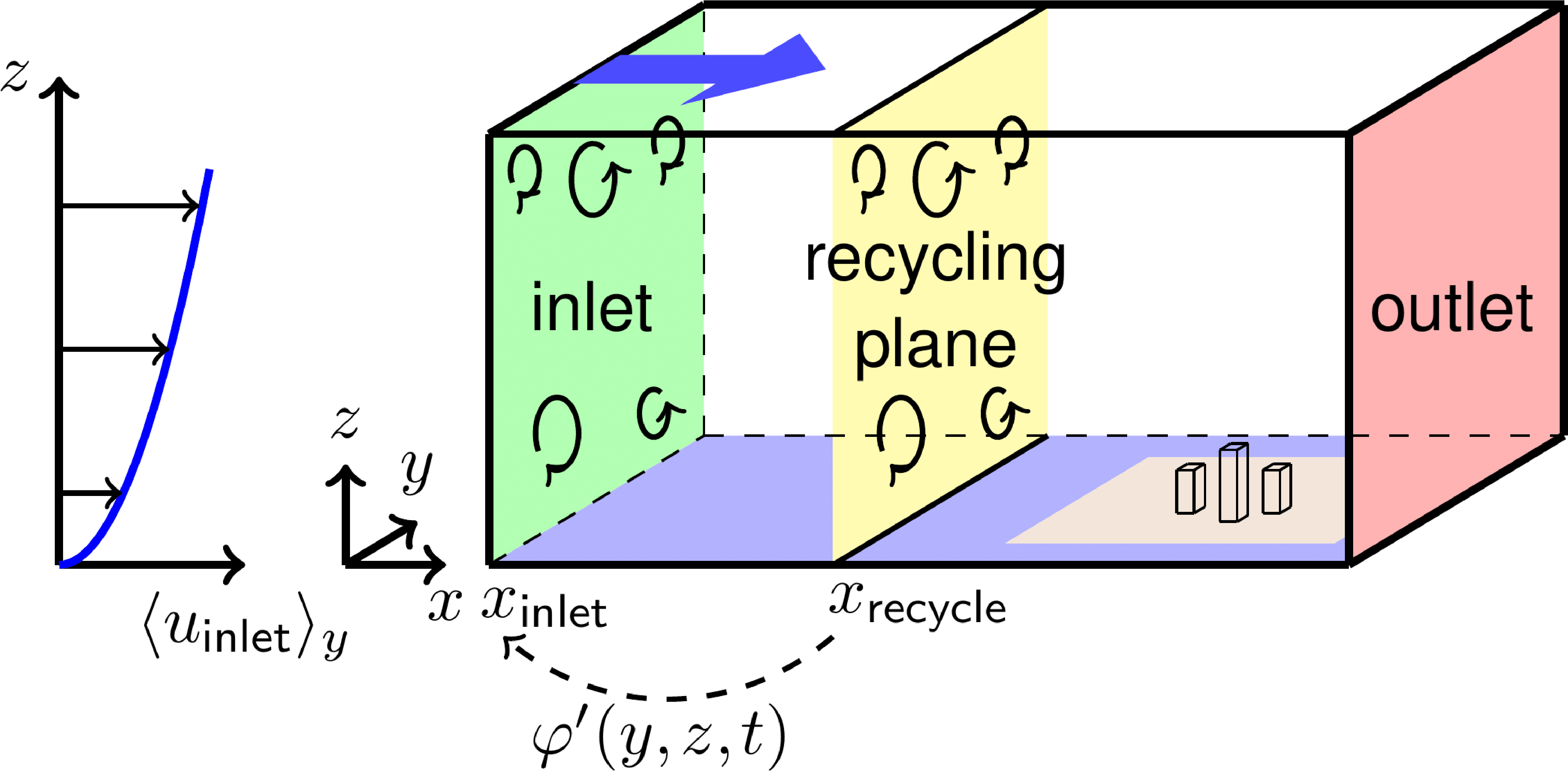
03.png
(465.4 KB) -
added by Giersch 9 years ago.
Turbulence recycling method
-
04.png
(91.3 KB) -
added by Giersch 9 years ago.
Sketch of the 2.5-D implementation of topography
-
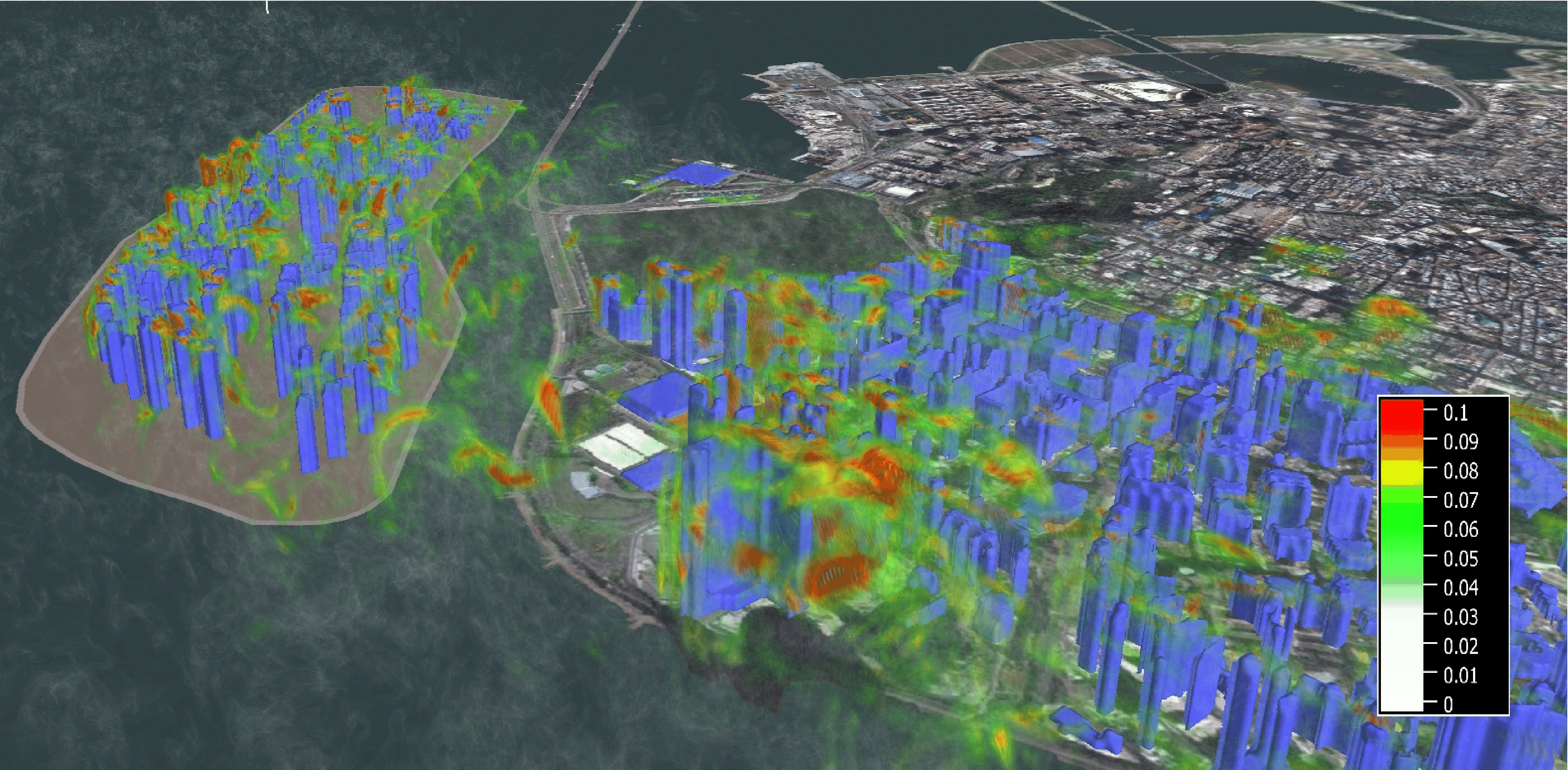
05.png
(5.0 MB) -
added by Giersch 9 years ago.
Snapshot of turbulence structures induced by a densely built-up artificial island of the coast of Macau, China
-
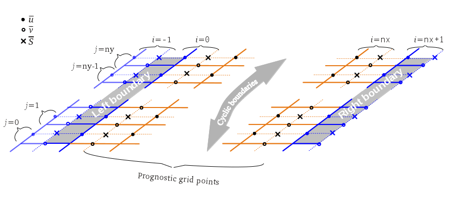
grid_lr.png
(89.4 KB) -
added by Giersch 9 years ago.
Grid structure at the lateral boundaries with non-cyclic lateral boundary conditions along the left-right direction
-
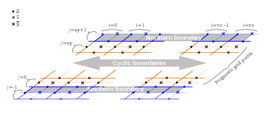
grid_ns.png
(74.7 KB) -
added by Giersch 9 years ago.
Figure 2: Grid structure of the lateral boundaries with non-cyclic lateral boundary conditions along the north-south direction.
- mask_method.png (19.6 KB) - added by suehring 8 years ago.