Initialization parameters ¶

Mode ¶

Grid ¶

Numerics ¶

Physics ¶

Boundary Conditions ¶

Initialization ¶

Topography ¶

Canopy ¶

Others ¶

NAMELIST group name: inipar

---

Mode: ¶

Parameter Name	FORTRAN Type	Default Value	Explanation
cloud_droplets ¶	L	.F.	Parameter to switch on usage of cloud droplets. Cloud droplets require to use particles (i.e. the NAMELIST group particles_par has to be included in the parameter file). Then each particle is a representative for a certain number of droplets. The droplet features (number of droplets, initial radius, etc.) can be steered with the respective particle parameters (see e.g. radius). The real number of initial droplets in a grid cell is equal to the initial number of droplets (defined by the particle source parameters pst, psl, psr, pss, psn, psb, pdx, pdy and pdz) times the initial_weighting_factor. In case of using cloud droplets, the default condensation scheme in PALM cannot be used, i.e. cloud_physics must be set .F..
cloud_physics ¶	L	.F.	Parameter to switch on the condensation scheme. For cloud_physics = .T., equations for the liquid water content and the liquid water potential temperature are solved instead of those for specific humidity and potential temperature. Note that a grid volume is assumed to be either completely saturated or completely unsaturated (0%-or-100%-scheme). A simple precipitation scheme can additionally be switched on with parameter precipitation. Also cloud-top cooling by longwave radiation can be utilized (see radiation). cloud_physics = .T. requires humidity = .T.. Detailed information about the condensation scheme is given in the description of the cloud physics module? (pdf-file, only in German). This condensation scheme is not allowed if cloud droplets are simulated explicitly (see cloud_droplets).
conserve_volume_flow ¶	L	.F.	Conservation of volume flow in x- and y-direction. conserve_volume_flow = .T. guarantees that the volume flow through the xz- and yz-cross-sections of the total model domain remains constant throughout the run depending on the chosen conserve_volume_flow_mode. Note that conserve_volume_flow = .T. requires dp_external = .F..
conserve_volume_flow_mode ¶	C*16	'default'	Modus of volume flow conservation. The following values are allowed: 'default' Per default, PALM uses 'initial_profiles' for cyclic lateral boundary conditions (bc_lr = 'cyclic' and bc_ns = 'cyclic') and 'inflow_profile' for non-cyclic lateral boundary conditions (bc_lr /= 'cyclic' or bc_ns /= 'cyclic'). 'initial_profiles' The target volume flow is calculated at t=0 from the initial profiles of u and v. This setting is only allowed for cyclic lateral boundary conditions (bc_lr = 'cyclic' and bc_ns = 'cyclic'). 'inflow_profile' The target volume flow is calculated at every timestep from the inflow profile of u or v, respectively. This setting is only allowed for non-cyclic lateral boundary conditions (bc_lr /= 'cyclic' or bc_ns /= 'cyclic'). 'bulk_velocity' The target volume flow is calculated from a predefined bulk velocity (see u_bulk and v_bulk). This setting is only allowed for cyclic lateral boundary conditions (bc_lr = 'cyclic' and bc_ns = 'cyclic'). Note that conserve_volume_flow_mode only comes into effect if conserve_volume_flow = .T..
coupling_start_time ¶	R	0.0	Simulation time of precursor run. Sets the time period a precursor run shall run uncoupled. This parameter is used to set up the precursor run control for atmosphere-ocean-coupled runs. It has to be set individually to the atmospheric / oceanic precursor run. The time in the data output will show negative values during the precursor run. See documentation for further information.
dp_external ¶	L	.F.	External pressure gradient switch. This parameter is used to switch on/off an external pressure gradient as driving force. The external pressure gradient is controlled by the parameters dp_smooth, dp_level_b and dpdxy. Note that dp_external = .T. requires conserve_volume_flow = .F.. It is normally recommended to disable the Coriolis force by setting omega = 0.0.
dp_smooth ¶	L	.F.	Vertically smooth the external pressure gradient using a sinusoidal smoothing function. This parameter only applies if dp_external = .T.. It is useful in combination with dp_level_b >> 0 to generate a non-accelerated boundary layer well below dp_level_b.
dp_level_b ¶	R	0.0	Lower limit of the vertical range for which the external pressure gradient is applied (in m). This parameter only applies if dp_external = .T.. It must hold the condition zu(0) <= dp_level_b <= zu(nz). It can be used in combination with dp_smooth = .T. to generate a non-accelerated boundary layer well below dp_level_b if dp_level_b >> 0. Note that there is no upper limit of the vertical range because the external pressure gradient is always applied up to the top of the model domain.
dpdxy ¶	R(2)	2 * 0.0	Values of the external pressure gradient applied in x- and y-direction, respectively (in Pa/m). This parameter only applies if dp_external = .T.. It sets the pressure gradient values. Negative values mean an acceleration, positive values mean deceleration. For example, dpdxy = -0.0002, 0.0, drives the flow in positive x-direction.
e_init ¶	R	0.0	Initial subgrid-scale TKE in m2s-2. This option prescribes an initial subgrid-scale TKE from which the initial diffusion coefficients Km and Kh will be calculated if e_init is positive. This option only has an effect if km_constant is not set.
e_min ¶	R	0.0	Minimum subgrid-scale TKE in m2s-2. This option adds artificial viscosity to the flow by ensuring that the subgrid-scale TKE does not fall below the minimum threshold e_min.
galilei_transformation ¶	L	.F.	Application of a Galilei-transformation to the coordinate system of the model. With galilei_transformation = .T., a so-called Galilei-transformation is switched on which ensures that the coordinate system of the model is moved along with the geostrophical wind. Alternatively, the model domain can be moved along with the averaged horizontal wind (see use_ug_for_galilei_tr, this can and will naturally change in time). With this method, numerical inaccuracies of the Piascek - Williams - scheme (concerns in particular the momentum advection) are minimized. Beyond that, in the majority of cases the lower relative velocities in the moved system permit a larger time step (dt). Switching the transformation on is only worthwhile if the geostrophical wind (ug, vg) and the averaged horizontal wind clearly deviate from the value 0. In each case, the distance the coordinate system has been moved is written to the file RUN_CONTROL. Non-cyclic lateral boundary conditions (see bc_lr and bc_ns), the specification of a gestrophic wind that is not constant with height as well as e.g. stationary inhomogeneities at the bottom boundary do not allow the use of this transformation.
humidity ¶	L	.F.	Parameter to switch on the prognostic equation for specific humidity q. The initial vertical profile of q can be set via parameters q_surface, q_vertical_gradient and q_vertical_gradient_level. Boundary conditions can be set via q_surface_initial_change and surface_waterflux. If the condensation scheme is switched on (cloud_physics = .T.), q becomes the total liquid water content (sum of specific humidity and liquid water content).
km_constant ¶	R	variable (computed from TKE)	Constant eddy diffusivities are used (laminar simulations). If this parameter is specified, both in the 1d and in the 3d-model constant values for the eddy diffusivities are used in space and time with Km = km_constant and Kh = Km / prandtl_number?. The prognostic equation for the subgrid-scale TKE is switched off. Constant eddy diffusivities are only allowed with the Prandtl layer (prandtl_layer) switched off.
km_damp_max ¶	R	0.5*(dx or dy)	Maximum diffusivity used for filtering the velocity field in the vicinity of the outflow (in m2/s). When using non-cyclic lateral boundaries (see bc_lr or bc_ns), a smoothing has to be applied to the velocity field in the vicinity of the outflow in order to suppress any reflections of outgoing disturbances. Smoothing is done by increasing the eddy diffusivity along the horizontal direction which is perpendicular to the outflow boundary. Only velocity components parallel to the outflow boundary are filtered (e.g. v and w, if the outflow is along x). Damping is applied from the bottom to the top of the domain. The horizontal range of the smoothing is controlled by outflow_damping_width which defines the number of gridpoints (counted from the outflow boundary) from where on the smoothing is applied. Starting from that point, the eddy diffusivity is linearly increased (from zero to its maximum value given by km_damp_max) until half of the damping range width, from where it remains constant up to the outflow boundary. If at a certain grid point the eddy diffusivity calculated from the flow field is larger than as described above, it is used instead. The default value of km_damp_max has been empirically proven to be sufficient.
ocean ¶	L	.F.	Parameter to switch on ocean runs. By default PALM is configured to simulate atmospheric flows. However, starting from version 3.3, ocean = .T. allows simulation of ocean turbulent flows. Setting this switch has several effects: An additional prognostic equation for salinity is solved. Potential temperature in buoyancy and stability-related terms is replaced by potential density. Potential density is calculated from the equation of state for seawater after each timestep, using the algorithm proposed by Jackett et al. (2006, J. Atmos. Oceanic Technol., 23, 1709-1728). So far, only the initial hydrostatic pressure is entered into this equation. z=0 (sea surface) is assumed at the model top (vertical grid index k=nzt on the w-grid), with negative values of z indicating the depth. Initial profiles are constructed (e.g. from pt_vertical_gradient / pt_vertical_gradient_level) starting from the sea surface, using surface values given by pt_surface, sa_surface, ug_surface, and vg_surface. Zero salinity flux is used as default boundary condition at the bottom of the sea. If switched on, random perturbations are by default imposed to the upper model domain from zu(nzt*2/3) to zu(nzt-3). Relevant parameters to be exclusively used for steering ocean runs are bc_sa_t, bottom_salinityflux, sa_surface, sa_vertical_gradient, sa_vertical_gradient_level, and top_salinityflux. Section 4.4.2? gives an example for appropriate settings of these and other parameters neccessary for ocean runs. ocean = .T. does not allow settings of timestep_scheme = 'leapfrog' or 'leapfrog+euler' as well as scalar_advec = 'ups-scheme'.
passive_scalar ¶	L	.F.	Parameter to switch on the prognostic equation for a passive scalar. The initial vertical profile of s can be set via parameters s_surface, s_vertical_gradient and s_vertical_gradient_level. Boundary conditions can be set via s_surface_initial_change and surface_scalarflux. Note: With passive_scalar switched on, the simultaneous use of humidity (see humidity) is impossible.
precipitation ¶	L	.F.	Parameter to switch on the precipitation scheme. For precipitation processes PALM uses a simplified Kessler scheme. This scheme only considers the so-called autoconversion, that means the generation of rain water by coagulation of cloud drops among themselves. Precipitation begins and is immediately removed from the flow as soon as the liquid water content exceeds the critical value of 0.5 g/kg. The precipitation rate and amount can be output by assigning the runtime parameter data_output = 'prr*' or 'pra*', respectively. The time interval on which the precipitation amount is defined can be controlled via runtime parameter precipitation_amount_interval.
radiation ¶	L	.F.	Parameter to switch on longwave radiation cooling at cloud-tops. Long-wave radiation processes are parameterized by the effective emissivity, which considers only the absorption and emission of long-wave radiation at cloud droplets. The radiation scheme can be used only with cloud_physics = .TRUE..
random_heatflux ¶	L	.F.	Parameter to impose random perturbations on the internal two-dimensional near surface heat flux field shf. If a near surface heat flux is used as bottom boundary condition (see surface_heatflux), it is by default assumed to be horizontally homogeneous. Random perturbations can be imposed on the internal two-dimensional heat flux field shf by assigning random_heatflux = .T.. The disturbed heat flux field is calculated by multiplying the values at each mesh point with a normally distributed random number with a mean value and standard deviation of 1. This is repeated after every timestep. In case of a non-flat topography, assigning random_heatflux = .T. imposes random perturbations on the combined heat flux field shf composed of surface_heatflux at the bottom surface and wall_heatflux(0) at the topography top face.
u_bulk ¶	R	0.0	u-component of the predefined bulk velocity (in m/s). This parameter comes into effect if conserve_volume_flow = .T. and conserve_volume_flow_mode = 'bulk_velocity'.
use_ug_for_galilei_tr ¶	L	.T.	Switch to determine the translation velocity in case that a Galilean transformation is used. In case of a Galilean transformation (see galilei_transformation), use_ug_for_galilei_tr = .T. ensures that the coordinate system is translated with the geostrophic windspeed. Alternatively, with use_ug_for_galilei_tr = .F., the geostrophic wind can be replaced as translation speed by the (volume) averaged velocity. However, in this case the user must be aware of fast growing gravity waves, so this choice is usually not recommended!
v_bulk ¶	R	0.0	v-component of the predefined bulk velocity (in m/s). This parameter comes into effect if conserve_volume_flow = .T. and conserve_volume_flow_mode = 'bulk_velocity'.
ws_vertical_gradient ¶	R(10)	10 * 0.0	Gradient(s) of the profile for the large scale subsidence/ascent velocity (in (m/s) / 100 m). This gradient holds starting from the height level defined by ws_vertical_gradient_level (precisely: for all uv levels k where zu(k) > ws_vertical_gradient_level, w_subs(k) is set: w_subs(k) = w_subs(k-1) + dzu(k) * ws_vertical_gradient) up to the top boundary or up to the next height level defined by ws_vertical_gradient_level. A total of 10 different gradients for 11 height intervals (10 intervals if ws_vertical_gradient_level(1) = 0.0) can be assigned. Example: ws_vertical_gradient = -0.002, 0.0, ws_vertical_gradient_level = 0.0, 1000.0, That defines the subsidence/ascent profile to be linear up to z = 1000.0 m with a surface value of 0 m/s. For z > 1000.0 m up to the top boundary the gradient is 0.0 (m/s) / 100 m (it is assumed that the assigned height levels correspond with uv levels). With an appropriate construction of w_subs the height of the boundary layer z_i can be kept approximately constant. Attention: The large scale vertical motion is only applied to the prognostic equation for the scalar quantities (potential temperature, humidity if humidity = .T. or passive scalar if passive_scalar = .T.) because it cannot be applied to the momentum equations due to incompressibility. Thus, the model is not mass consistent.
[=#ws_vertical_gradient _level ws_vertical_gradient _level]	R(10)	10 * 0.0	Height level from which on the gradient for the subsidence/ascent velocity defined by ws_vertical_gradient is effective (in m). The height levels have to be assigned in ascending order. The default values result in a profile which is zero everywhere regardless of the values of ws_vertical_gradient. For the piecewise construction of the subsidence/ascent velocity profile see ws_vertical_gradient.

Grid: ¶

Parameter Name	FORTRAN Type	Default Value	Explanation
dx ¶	R	1.0	Horizontal grid spacing along the x-direction (in m). Along x-direction only a constant grid spacing is allowed. For coupled runs (see 3.8?) this parameter must be equal in both parameter files PARIN and PARIN_O.
dy ¶	R	1.0	Horizontal grid spacing along the y-direction (in m). Along y-direction only a constant grid spacing is allowed. For coupled runs (see 3.8?) this parameter must be equal in both parameter files PARIN and PARIN_O.
dz ¶	R		Vertical grid spacing (in m). This parameter must be assigned by the user, because no default value is given. By default, the model uses constant grid spacing along z-direction, but it can be stretched using the parameters dz_stretch_level and dz_stretch_factor. In case of stretching, a maximum allowed grid spacing can be given by dz_max. Assuming a constant dz, the scalar levels (zu) are calculated directly by: zu(0) = - dz * 0.5 zu(1) = dz * 0.5 The w-levels lie half between them: zw(k) = ( zu(k) + zu(k+1) ) * 0.5
dz_max ¶	R	9999999.9	Allowed maximum vertical grid spacing (in m). If the vertical grid is stretched (see dz_stretch_factor and dz_stretch_level), dz_max can be used to limit the vertical grid spacing.
dz_stretch_factor ¶	R	1.08	Stretch factor for a vertically stretched grid (see dz_stretch_level). The stretch factor should not exceed a value of approx. 1.10 - 1.12, otherwise the discretization errors due to the stretched grid are not negligible any more. (refer Kalnay de Rivas)
dz_stretch_level ¶	R	100000.0	Height level above/below which the grid is to be stretched vertically (in m). For ocean = .F., dz_stretch_level is the height level (in m) above which the grid is to be stretched vertically. The vertical grid spacings dz above this level are calculated as dz(k+1) = dz(k) * dz_stretch_factor and used as spacings for the scalar levels (zu). The w-levels are then defined as: zw(k) = ( zu(k) + zu(k+1) ) * 0.5. For ocean = .T., dz_stretch_level is the height level (in m, negative) below which the grid is to be stretched vertically. The vertical grid spacings dz below this level are calculated correspondingly as dz(k-1) = dz(k) * dz_stretch_factor.
grid_matching ¶	C*6	'strict'	Variable to adjust the subdomain sizes in parallel runs. For grid_matching = 'strict' , the subdomains are forced to have an identical size on all processors. In this case the processor numbers in the respective directions of the virtual processor net must fulfill certain divisor conditions concerning the grid point numbers in the three directions (see nx, ny and nz). Advantage of this method is that all PEs bear the same computational load. There is no such restriction by default, because then smaller subdomains are allowed on those processors which form the right and/or north boundary of the virtual processor grid. On all other processors the subdomains are of same size. Whether smaller subdomains are actually used, depends on the number of processors and the grid point numbers used. Information about the respective settings are given in file RUN_CONTROL. When using a multi-grid method for solving the Poisson equation (see psolver) only grid_matching = 'strict' is allowed. Note: In some cases for small processor numbers there may be a very bad load balancing among the processors which may reduce the performance of the code.
npex ¶	I		Number of processors along x-direction of the virtual processor net. For parallel runs, the total number of processors to be used is given by the mrun-option -X. By default, depending on the type of the parallel computer, PALM generates a 1d processor net (domain decomposition along x, npey = 1) or a 2d-net (this is favored on machines with fast communication network and/or large number of processors (>256)). In case of a 2d-net, it is tried to make it more or less square-shaped. If, for example, 16 processors are assigned (-X 16), a 4 * 4 processor net is generated (npex = 4, npey = 4). This choice is optimal for square total domains (nx = ny), since then the number of ghost points at the lateral boundarys of the subdomains reaches a minimum. If nx and ny differ extremely, the processor net should be manually adjusted using adequate values for npex and npey. Important: The value of npex * npey must exactly match the value assigned by the mrun-option -X. Otherwise the model run will abort with a corresponding error message. Additionally, the specification of npex and npey may of course override the default setting for the domain decomposition (1d or 2d) which may have a significant (negative) effect on the code performance.
npey ¶	I		Number of processors along y-direction of the virtual processor net. For further information see npex.
nx ¶	I		Number of grid points in x-direction. A value for this parameter must be assigned. Since the lower array bound in PALM starts with i = 0, the actual number of grid points is equal to nx+1. In case of cyclic boundary conditions along x, the domain size is (nx+1)* dx. For parallel runs, in case of grid_matching = 'strict', nx+1 must be an integral multiple of the processor numbers (see npex and npey) along x- as well as along y-direction (due to data transposition restrictions). For coupled runs this parameter must be equal in both parameter files PARIN and PARIN_O.
ny ¶	I		Number of grid points in y-direction. A value for this parameter must be assigned. Since the lower array bound in PALM starts with j = 0, the actual number of grid points is equal to ny+1. In case of cyclic boundary conditions along y, the domain size is (ny+1) * dy. For parallel runs, in case of grid_matching = 'strict', ny+1 must be an integral multiple of the processor numbers (see npex and npey) along y- as well as along x-direction (due to data transposition restrictions). For coupled runs this parameter must be equal in both parameter files PARIN and PARIN_O.
nz ¶	I		Number of grid points in z-direction. A value for this parameter must be assigned. Since the lower array bound in PALM starts with k = 0 and since one additional grid point is added at the top boundary (k = nz+1), the actual number of grid points is nz+2. However, the prognostic equations are only solved up to nz (u, v) or up to nz-1 (w, scalar quantities). The top boundary for u and v is at k = nz+1 (u, v) while at k = nz for all other quantities. For parallel runs, in case of grid_matching = 'strict', nz must be an integral multiple of the number of processors in x-direction (due to data transposition restrictions).
nz_do3d ¶	I	nz+1	Limits the output of 3d volume data along the vertical direction (grid point index k). By default, data for all grid points along z are output. The parameter nz_do3d can be used to limit the output up to a certain vertical grid point (e.g. in order to reduce the amount of output data). It affects all output of volume data ("normal" output to file, see data_output, as well as output for dvrp-software, see mode_dvrp).
[=#<insert_parameter_name> <insert_parameter_name>]	<insert type>	<insert value>	<insert explanation>
[=#<insert_parameter_name> <insert_parameter_name>]	<insert type>	<insert value>	<insert explanation>

Numerics: ¶

Parameter Name	FORTRAN Type	Default Value	Explanation
call_psolver_at_all_substeps ¶	L	.T.	Switch to steer the call of the pressure solver. In order to speed-up performance, the Poisson equation for perturbation pressure (see psolver) can be called only at the last substep of multistep Runge-Kutta timestep schemes (see timestep_scheme) by setting call_psolver_at_all_substeps = .F.. In many cases, this sufficiently reduces the divergence of the velocity field. Nevertheless, small-scale ripples (2-delta-x) may occur. In this case and in case of non-cyclic lateral boundary conditions, call_psolver_at_all_timesteps = .T. should be used.
cfl_factor ¶	R	0.1, 0.8 or 0.9 (see right)	Time step limiting factor. In the model, the maximum allowed time step according to CFL and diffusion-criterion dt_max is reduced by dt = dt_max * cfl_factor in order to avoid stability problems which may arise in the vicinity of the maximum allowed timestep. The condition 0.0 < cfl_factor < 1.0 applies. The default value of cfl_factor depends on the timestep_scheme used: For the third order Runge-Kutta scheme it is cfl_factor = 0.9. In case of the leapfrog scheme a quite restrictive value of cfl_factor = 0.1 is used because for larger values the velocity divergence significantly effects the accuracy of the model results. Possibly larger values may be used with the leapfrog scheme but these are to be determined by appropriate test runs. The default value for the Euler scheme is cfl_factor = 0.8.
cycle_mg ¶	C*1	'w'	Type of cycle to be used with the multi-grid method. This parameter determines which type of cycle is applied in the multi-grid method used for solving the Poisson equation for perturbation pressure (see psolver). It defines in which way it is switched between the fine and coarse grids. So-called v- and w-cycles are realized (i.e. cycle_mg may be assigned the values 'v' or 'w' ). The computational cost of w-cycles is much higher than that of v-cycles, however, w-cycles give a much better convergence.
fft_method ¶	C*20	'system-specific'	FFT-method to be used. The fast fourier transformation (FFT) is used for solving the perturbation pressure equation with a direct method (see psolver) and for calculating power spectra (see optional software packages, 4.2?). By default, system-specific, optimized routines from external vendor libraries are used. However, these are available only on certain computers and there are more or less severe restrictions concerning the number of gridpoints to be used with them. There are two other PALM internal methods available on every machine (their respective source code is part of the PALM source code): 1.: The Temperton-method from Clive Temperton (ECWMF) which is computationally very fast and switched on with fft_method = 'temperton-algorithm'. The number of horizontal gridpoints (nx+1, ny+1) to be used with this method must be composed of prime factors 2, 3 and 5. 2.: The Singleton-method which is very slow but has no restrictions concerning the number of gridpoints to be used with, switched on with fft_method = 'singleton-algorithm'.
long_filter_factor ¶	R	0.0	Filter factor for the so-called Long-filter. This filter very efficiently eliminates 2-delta-waves sometimes caused by the upstream-spline scheme (see Mahrer and Pielke, 1978: Mon. Wea. Rev., 106, 818-830). It works in all three directions in space. A value of long_filter_factor = 0.01 sufficiently removes the small-scale waves without affecting the longer waves. By default, the filter is switched off (= 0.0). It is exclusively applied to the tendencies calculated by the upstream-spline scheme (see momentum_advec and scalar_advec), not to the prognostic variables themselves. At the bottom and top boundary of the model domain the filter effect for vertical 2-delta-waves is reduced. There, the amplitude of these waves is only reduced by approx. 50%, otherwise by nearly 100%. Filter factors with values > 0.01 also reduce the amplitudes of waves with wavelengths longer than 2-delta (see the paper by Mahrer and Pielke, quoted above).
loop_optimization ¶	C*16	see right	Method used to optimize loops for solving the prognostic equations. By default, the optimization method depends on the host on which PALM is running. On machines with vector-type CPUs, single 3d-loops are used to calculate each tendency term of each prognostic equation, while on all other machines, all prognostic equations are solved within one big loop over the two horizontal indices i and j (giving a good cache uitilization). The default behaviour can be changed by setting either loop_optimization = 'vector' or loop_optimization = 'cache'.
mg_cycles ¶	I	-1	Number of cycles to be used with the multi-grid scheme. This parameter determines the number of cycles to be carried out in the multi-grid method used for solving the Poisson equation for perturbation pressure (see psolver). The type of the cycles can be set with cycle_mg. By default (mg_cyles = -1), the number of cycles depends on the requested accuracy of the scheme (see residual_limit) and may vary from time step to time step. In this case, the CPU time for a run will be difficult to estimate, since it heavily depends on the total number of the cycles to be carried out. By assigning mg_cycles a value (>= 1), the number of cycles can be fixed so that the CPU time can be clearly estimated. Note: When using a fixed number of cycles, the user must examine the local file RUN_CONTROL regularly to check whether the divergence of the velocity field is sufficiently reduced by the pressure solver. It should be reduced at least by two orders of magnitude. For cyclic boundary conditions along both horizontal directions (see bc_lr and bc_ns) mg_cycles = 2 is typically a good choice, for non-cyclic lateral boundary conditions mg_cycles = 4 may be sufficient.
mg_switch_to_pe0_level ¶	I		Grid level at which data shall be gathered on PE0. In case of a run using several PEs and the multigrid method for solving the Poisson equation for perturbation pressure (see psolver), the value of this parameter defines on which grid level the data are gathered on PE0 in order to allow for a further coarsening of the grid. The finest grid defines the largest grid level. By default, the gathering level is determined automatically and displayed in file RUN_CONTROL. It is only possible to gather data from a level larger than the one determined automatically. A test run may be neccessary to determine this level. Setting of mg_switch_to_pe0_level = -1 prevents that data are collected on PE0 at all, i.e. coarsening of grids is limited by the subdomains.
momentum_advec ¶	C*10	'pw-scheme'	Advection scheme to be used for the momentum equations. The user can choose between the following schemes: 'pw-scheme' The scheme of Piascek and Williams (1970, J. Comp. Phys., 6, 392-405) with central differences in the form C3 is used. If intermediate Euler-timesteps are carried out in case of timestep_scheme = 'leapfrog+euler' the advection scheme is - for the Euler-timestep - automatically switched to an upstream-scheme. 'ups-scheme' The upstream-spline scheme is used (see Mahrer and Pielke, 1978: Mon. Wea. Rev., 106, 818-830). In opposite to the Piascek-Williams scheme, this is characterized by much better numerical features (less numerical diffusion, better preservation of flow structures, e.g. vortices), but computationally it is much more expensive. In addition, the use of the Euler-timestep scheme is mandatory (timestep_scheme = 'euler' ), i.e. the timestep accuracy is only of first order. For this reason the advection of scalar variables (see scalar_advec) should then also be carried out with the upstream-spline scheme, because otherwise the scalar variables would be subject to large numerical diffusion due to the upstream scheme. Since the cubic splines used tend to overshoot under certain circumstances, this effect must be adjusted by suitable filtering and smoothing (see cut_spline_overshoot, long_filter_factor, ups_limit_pt, ups_limit_u, ups_limit_v, ups_limit_w). This is always neccessary for runs with stable stratification, even if this stratification appears only in parts of the model domain. With stable stratification the upstream-spline scheme also produces gravity waves with large amplitude, which must be suitably damped (see rayleigh_damping_factor). Important: The upstream-spline scheme is not implemented for humidity and passive scalars (see humidity and passive_scalar) and requires the use of a 2d-domain-decomposition. The last conditions severely restricts code optimization on several machines leading to very long execution times! The scheme is also not allowed for non-cyclic lateral boundary conditions (see bc_lr and bc_ns).
ngsrb ¶	I	2	Grid level at which data shall be gathered on PE0. In case of a run using several PEs and the multigrid method for solving the Poisson equation for perturbation pressure (see psolver), the value of this parameter defines on which grid level the data are gathered on PE0 in order to allow for a further coarsening of the grid. The finest grid defines the largest grid level. By default, the gathering level is determined automatically and displayed in file RUN_CONTROL. It is only possible to gather data from a level larger than the one determined automatically. A test run may be neccessary to determine this level.
nsor ¶	I	20	Number of iterations to be used with the SOR-scheme. This parameter is only effective if the SOR-scheme is selected as pressure solver (psolver = 'sor' ). The number of iterations necessary for a sufficient convergence of the scheme depends on the grid point numbers and is to be determined by appropriate test runs (the default value will not at all be sufficient for larger grid point numbers). The number of iterations used for the first call of the SOR-scheme (t = 0) is determined via the parameter nsor_ini.
nsor_ini ¶	I	100	Initial number of iterations with the SOR algorithm. This parameter is only effective if the SOR algorithm was selected as the pressure solver scheme (psolver = 'sor' ) and specifies the number of initial iterations of the SOR scheme (at t = 0). The number of subsequent iterations at the following timesteps is determined with the parameter nsor. Usually nsor < nsor_ini, since in each case subsequent calls to psolver use the solution of the previous call as initial value. Suitable test runs should determine whether sufficient convergence of the solution is obtained with the default value and if necessary the value of nsor_ini should be changed.
omega_sor ¶	R	1.8	Convergence factor to be used with the the SOR-scheme. If the SOR-scheme is selected (psolver = 'sor' ), this parameter determines the value of the convergence factor, where 1.0 <= omega_sor < 2.0. The optimum value of omega_sor depends on the number of grid points along the different directions in space. For non-equidistant grids it can only be determined by appropriate test runs.
psolver ¶	C*10	'poisfft'	Scheme to be used to solve the Poisson equation for the perturbation pressure. The user can choose between the following schemes: 'poisfft' Direct method using FFT along x and y, solution of a tridiagonal matrix along z, and backward FFT (see Siano, institute reports, volume 54). The FFT routines to be used can be determined via the initialization parameter fft_method. This solver is specially optimized for 1d domain decompositions. Vectorization is optimized for domain decompositions along x only. 'poisfft_hybrid' Direct method using FFT along x and y, solution of a tridiagonal matrix along z, and backward FFT (see Siano, institute reports, volume 54). The FFT routines to be used can be determined via the initialization parameter fft_method. This solver is specially optimized for 1d domain decompositions. Vectorization is optimized for domain decompositions along x only. 'multigrid' Multi-grid scheme (see Uhlenbrock, diploma thesis). v- and w-cycles (see cycle_mg) are implemented. The convergence of the iterative scheme can be steered by the number of v-/w-cycles to be carried out for each call of the scheme (mg_cycles) and by the number of Gauss-Seidel iterations (see ngsrb) to be carried out on each grid level. Instead the requested accuracy can be given via residual_limit. This is the default! The smaller this limit is, the more cycles have to be carried out in this case and the number of cycles may vary from timestep to timestep. If mg_cycles is set to its optimal value, the computing time of the multi-grid scheme amounts approximately to that of the direct solver 'poisfft', as long as the number of grid points in the three directions of space corresponds to a power-of-two (2n) where n >= 5 must hold. With large n, the multi-grid scheme can even be faster than the direct solver (although its accuracy is several orders of magnitude worse, but this does not affect the accuracy of the simulation). Nevertheless, the user should always carry out some test runs in order to find out the optimum value for mg_cycles, because the CPU time of a run very critically depends on this parameter. This scheme requires that the number of grid points of the subdomains (or of the total domain, if only one PE is uesd) along each of the directions can at least be devided once by 2 without rest. With parallel runs, starting from a certain grid level the data of the subdomains are possibly gathered on PE0 in order to allow for a further coarsening of the grid. The grid level for gathering can be manually set by mg_switch_to_pe0_level. Using this procedure requires the subdomains to be of identical size (see grid_matching). 'sor' Successive over relaxation method (SOR). The convergence of this iterative scheme is steered with the parameters omega_sor, nsor_ini and nsor. Compared to the direct method and the multi-grid method, this scheme needs substantially more computing time. It should only be used for test runs, e.g. if errors in the other pressure solver methods are assumed. In order to speed-up performance, the Poisson equation is by default only solved at the last substep of a multistep Runge-Kutta scheme (see at_all_substeps call_psolver at_all_substeps and timestep_scheme).
pt_reference ¶	R	use horizontal average as reference	Reference temperature to be used in all buoyancy terms (in K). By default, the instantaneous horizontal average over the total model domain is used. Attention: In case of ocean runs (see ocean), always a reference temperature is used in the buoyancy terms with a default value of pt_reference = pt_surface.
random_generator ¶	C*20	'numerical recipes'	Random number generator to be used for creating uniformly distributed random numbers. It is used if random perturbations are to be imposed on the velocity field or on the surface heat flux field (see create_disturbances and random_heatflux). By default, the "Numerical Recipes" random number generator is used. This one provides exactly the same order of random numbers on all different machines and should be used in particular for comparison runs. Besides, a system-specific generator is available ( random_generator = 'system-specific' ) which should particularly be used for runs on vector parallel computers (NEC), because the default generator cannot be vectorized and therefore significantly drops down the code performance on these machines. Note: Results from two otherwise identical model runs will not be comparable one-to-one if they used different random number generators.
rayleigh_damping_factor ¶	R	0.0 or 0.01	Factor for Rayleigh damping. A so-called Rayleigh damping is applied to all prognostic variables if a non-zero value is assigned to rayleigh_damping_factor. If switched on, variables are forced towards the value of their respective basic states (e.g. the geostrophic wind). The intensity of damping is controlled by the value the rayleigh_damping_factor is assigned to. The damping starts weakly at a height defined by rayleigh_damping_height and rises according to a sin2-function to its maximum value at the top (ocean: bottom) boundary. This method effectively damps gravity waves, caused by boundary layer convection, which may spread out vertically in the inversion layer and which are reflected at the top (ocean: bottom) boundary. This particularly happens with the upstream-spline scheme switched on (see momentum_advec or scalar_advec). Therefore, with this scheme the Rayleigh damping is switched on (rayleigh_damping_factor = 0.01) by default. Otherwise it remains switched off. The Rayleigh damping factor must hold the condition 0.0 <= rayleigh_damping_factor <= 1.0. Large values (close to 1.0) can cause numerical instabilities.
rayleigh_damping_height ¶	R	2/3 * zu(nz) \ (ocean: 2/3* zu(0))	Height above (ocean: below) which the Rayleigh damping starts (in m). With Rayleigh damping switched on (see rayleigh_damping_factor), this parameter determines the range where damping is applied. By default, Rayleigh damping will be applied in the upper (ocean: lower) third of the model domain.
residual_limit ¶	R	1.0E-6	Largest residual permitted for the multi-grid scheme (in s-2m-3). This is a parameter to steer the accuracy of the multi-grid scheme (see psolver). The assigned cycle (v- or w-cycle, see mg_cycles) is passed through until the residual falls below the limit given by residual_limit. If this is not the case after 1000 cycles, the PALM aborts with a corresponding error message. The reciprocal value of this parameter can be interpreted as a factor by the divergence of the provisional velocity field is approximately reduced after the multi-grid scheme has been applied (thus the default value causes a reduction of the divergence by approx. 6 orders of magnitude).
scalar_advec ¶	C*10	'pw-scheme'	Advection scheme to be used for the scalar quantities. The user can choose between the following schemes: 'pw-scheme' \ The scheme of Piascek and Williams (1970, J. Comp. Phys., 6, 392-405) with central differences in the form C3 is used. If intermediate Euler-timesteps are carried out in case of timestep_scheme = 'leapfrog+euler' the advection scheme is - for the Euler-timestep - automatically switched to an upstream-scheme. 'bc-scheme' \ The Bott scheme modified by Chlond (1994, Mon. Wea. Rev., 122, 111-125). This is a conservative monotonous scheme with very small numerical diffusion and therefore very good conservation of scalar flow features. The scheme however, is computationally very expensive both because it is expensive itself and because it does (so far) not allow specific code optimizations (e.g. cache optimization). Choice of this scheme forces the Euler timestep scheme to be used for the scalar quantities. For output of horizontally averaged profiles of the resolved / total heat flux, data_output_pr = 'w*pt*BC' / 'wptBC' should be used, instead of the standard profiles ( 'w*pt*' and 'wpt' ) because these are too inaccurate with this scheme. However, for subdomain analysis (see statistic_regions) exactly the reverse holds: here 'w*pt*BC' and 'wptBC' show very large errors and should not be used. This scheme is not allowed for non-cyclic lateral boundary conditions (see bc_lr and bc_ns). 'ups-scheme' \ The upstream-spline-scheme is used (see Mahrer and Pielke, 1978: Mon. Wea. Rev., 106, 818-830). In opposite to the Piascek Williams scheme, this is characterized by much better numerical features (less numerical diffusion, better preservation of flux structures, e.g. vortices), but computationally it is much more expensive. In addition, the use of the Euler-timestep scheme is mandatory (timestep_scheme = 'euler' ), i.e. the timestep accuracy is only first order. For this reason the advection of momentum (see momentum_advec) should then also be carried out with the upstream-spline scheme, because otherwise the momentum would be subject to large numerical diffusion due to the upstream scheme. Since the cubic splines used tend to overshoot under certain circumstances, this effect must be adjusted by suitable filtering and smoothing (see long_filter_factor). This is always neccesssary for runs with stable stratification, even if this stratification appears only in parts of the model domain. With stable stratification the upstream-upline scheme also produces gravity waves with large amplitude, which must be suitably damped (see rayleigh_damping_factor). Important: The upstream-spline scheme is not implemented for humidity and passive scalars (see humidity and passive_scalar) and requires the use of a 2d-domain-decomposition. The last conditions severely restricts code optimization on several machines leading to very long execution times! This scheme is also not allowed for non-cyclic lateral boundary conditions (see bc_lr and bc_ns). A differing advection scheme can be chosen for the subgrid-scale TKE using parameter use_upstream_for_tke.
[=#<insert_parameter_name> <insert_parameter_name>]	<insert type>	<insert value>	<insert explanation>
[=#<insert_parameter_name> <insert_parameter_name>]	<insert type>	<insert value>	<insert explanation>
[=#<insert_parameter_name> <insert_parameter_name>]	<insert type>	<insert value>	<insert explanation>
[=#<insert_parameter_name> <insert_parameter_name>]	<insert type>	<insert value>	<insert explanation>

Physics: ¶

Parameter Name	FORTRAN Type	Default Value	Explanation
omega ¶	R	7.29212E-5	Angular velocity of the rotating system (in rad s-1). The angular velocity of the earth is set by default. The values of the Coriolis parameters are calculated as: f = 2.0 * omega * sin(phi) f* = 2.0 * omega * cos(phi)
phi ¶	R	55.0	Geographical latitude (in degrees). The value of this parameter determines the value of the Coriolis parameters f and f*, provided that the angular velocity (see omega) is non-zero.
prandtl_number ¶	R	1.0	Ratio of the eddy diffusivities for momentum and heat (Km/Kh). For runs with constant eddy diffusivity (see km_constant), this parameter can be used to assign the Prandtl number (ratio Km / Kh).

Boundary Conditions: ¶

Parameter Name	FORTRAN Type	Default Value	Explanation
adjust_mixing_length ¶	L	.F.	Near-surface adjustment of the mixing length to the Prandtl-layer law. Usually the mixing length in LES models lLES depends (as in PALM) on the grid size and is possibly restricted further in case of stable stratification and near the lower wall (see parameter wall_adjustment). With adjust_mixing_length = .T. the Prandtl' mixing length lPR = kappa * z/phi is calculated and the mixing length actually used in the model is set l = MIN (lLES , lPR). This usually gives a decrease of the mixing length at the bottom boundary and considers the fact that eddy sizes decrease in the vicinity of the wall. Warning: So far, there is no good experience with adjust_mixing_length = .T.! With adjust_mixing_length = .T. and the Prandtl-layer being switched on (see prandtl_layer) '(u*)** 2+neumann' should always be set as the lower boundary condition for the TKE (see bc_e_b), otherwise the near-surface value of the TKE is not in agreement with the Prandtl-layer law (Prandtl-layer law and Prandtl-Kolmogorov-Ansatz should provide the same value for Km). A warning is given, if this is not the case.
bc_e_b ¶	C*20	'neumann'	Bottom boundary condition of the TKE. bc_e_b may be set to 'neumann' or '(u*)**2+neumann' . bc_e_b = 'neumann' yields to e(k=0)=e(k=1) (Neumann boundary condition), where e(k=1) is calculated via the prognostic TKE equation. Choice of '(u*)**2+neumann' also yields to e(k=0)=e(k=1), but the TKE at the Prandtl-layer top (k=1) is calculated diagnostically by e(k=1)=(us/0.1)**2. However, this is only allowed if a Prandtl-layer is used (prandtl_layer). If this is not the case, a warning is given and bc_e_b is reset to 'neumann' . At the top boundary a Neumann boundary condition is generally used: (e(nz+1) = e(nz)).
bc_lr ¶	C*20	'cyclic'	Boundary condition along x (for all quantities). By default, a cyclic boundary condition is used along x. bc_lr may also be assigned the values 'dirichlet/radiation' (inflow from left, outflow to the right) or 'radiation/dirichlet' (inflow from right, outflow to the left). This requires the multi-grid method to be used for solving the Poisson equation for perturbation pressure (see psolver) and it also requires cyclic boundary conditions along y (see bc_ns). In case of these non-cyclic lateral boundaries, a Dirichlet condition is used at the inflow for all quantities (initial vertical profiles - see initializing_actions - are fixed during the run) except u, to which a Neumann (zero gradient) condition is applied. At the outflow, a radiation condition is used for all velocity components, while a Neumann (zero gradient) condition is used for the scalars. For perturbation pressure Neumann (zero gradient) conditions are assumed both at the inflow and at the outflow. When using non-cyclic lateral boundaries, a filter is applied to the velocity field in the vicinity of the outflow in order to suppress any reflections of outgoing disturbances (see km_damp_max and outflow_damping_width). In order to maintain a turbulent state of the flow, it may be neccessary to continuously impose perturbations on the horizontal velocity field in the vicinity of the inflow throughout the whole run. This can be switched on using create_disturbances. The horizontal range to which these perturbations are applied is controlled by the parameters inflow_disturbance_begin and inflow_disturbance_end. The vertical range and the perturbation amplitude are given by disturbance_level_b, disturbance_level_t, and disturbance_amplitude. The time interval at which perturbations are to be imposed is set by dt_disturb. In case of non-cyclic horizontal boundaries call_psolver_at_all_substeps = .T. should be used. Note: Using non-cyclic lateral boundaries requires very sensitive adjustments of the inflow (vertical profiles) and the bottom boundary conditions, e.g. a surface heating should not be applied near the inflow boundary because this may significantly disturb the inflow. Please check the model results very carefully.
bc_ns ¶	C*20	'cyclic'	Boundary condition along y (for all quantities). By default, a cyclic boundary condition is used along y. bc_ns may also be assigned the values 'dirichlet/radiation' (inflow from rear ("north"), outflow to the front ("south")) or 'radiation/dirichlet' (inflow from front ("south"), outflow to the rear ("north")). This requires the multi-grid method to be used for solving the Poisson equation for perturbation pressure (see psolver) and it also requires cyclic boundary conditions along x (see bc_lr). In case of these non-cyclic lateral boundaries, a Dirichlet condition is used at the inflow for all quantities (initial vertical profiles - see initializing_actions - are fixed during the run) except u, to which a Neumann (zero gradient) condition is applied. At the outflow, a radiation condition is used for all velocity components, while a Neumann (zero gradient) condition is used for the scalars. For perturbation pressure Neumann (zero gradient) conditions are assumed both at the inflow and at the outflow. For further details regarding non-cyclic lateral boundary conditions see bc_lr.
bc_p_b ¶	C*20	'neumann'	Bottom boundary condition of the perturbation pressure. Allowed values are 'dirichlet' , 'neumann' and 'neumann+inhomo' . 'dirichlet' sets p(k=0)=0.0, 'neumann' sets p(k=0)=p(k=1). 'neumann+inhomo' corresponds to an extended Neumann boundary condition where heat flux or temperature inhomogeneities near the surface (pt(k=1)) are additionally regarded (see Shen and LeClerc? (1995, Q.J.R. Meteorol. Soc., 1209)). This condition is only permitted with the Prandtl-layer switched on (prandtl_layer), otherwise the run is terminated. Since at the bottom boundary of the model the vertical velocity disappears (w(k=0) = 0.0), the consistent Neumann condition ( 'neumann' or 'neumann+inhomo' ) dp/dz = 0 should be used, which leaves the vertical component w unchanged when the pressure solver is applied. Simultaneous use of the Neumann boundary conditions both at the bottom and at the top boundary (bc_p_t) usually yields no consistent solution for the perturbation pressure and should be avoided.
bc_p_t ¶	C*20	'dirichlet'	Top boundary condition of the perturbation pressure. Allowed values are 'dirichlet' (p(k=nz+1)= 0.0) or 'neumann' (p(k=nz+1)=p(k=nz)). Simultaneous use of Neumann boundary conditions both at the top and bottom boundary (bc_p_b) usually yields no consistent solution for the perturbation pressure and should be avoided. Since at the bottom boundary the Neumann condition is a good choice (see bc_p_b), a Dirichlet condition should be set at the top boundary.
bc_pt_b ¶	C*20	'dirichlet'	Bottom boundary condition of the potential temperature. Allowed values are 'dirichlet' (pt(k=0) = const. = pt_surface + pt_surface_initial_change; the user may change this value during the run using #user-defined code) and 'neumann' (pt(k=0)=pt(k=1)). When a constant surface sensible heat flux is used (surface_heatflux), bc_pt_b = 'neumann' must be used, because otherwise the resolved scale may contribute to the surface flux so that a constant value cannot be guaranteed. In the coupled atmosphere executable, bc_pt_b is internally set and does not need to be prescribed.
bc_pt_t ¶	C*20	'initial_gradient'	Top boundary condition of the potential temperature. Allowed are the values 'dirichlet' (pt(k=nz+1) does not change during the run), 'neumann' (pt(k=nz+1)=pt(k=nz)), and 'initial_gradient' . With the 'initial_gradient' -condition the value of the temperature gradient at the top is calculated from the initial temperature profile (see pt_surface, pt_vertical_gradient) by bc_pt_t_val = (pt_init(k=nz+1) - pt_init(k=nz)) / dzu(nz+1). Using this value (assumed constant during the run) the temperature boundary values are calculated as pt(k=nz+1) = pt(k=nz) + bc_pt_t_val * dzu(nz+1) (up to k=nz the prognostic equation for the temperature is solved). When a constant sensible heat flux is used at the top boundary (top_heatflux), bc_pt_t = 'neumann' must be used, because otherwise the resolved scale may contribute to the top flux so that a constant value cannot be guaranteed.
bc_q_b ¶	C*20	'dirichlet'	Bottom boundary condition of the specific humidity / total water content. Allowed values are 'dirichlet' (q(k=0) = const. = q_surface + q_surface_initial_change; the user may change this value during the run using #user-defined code) and 'neumann' (q(k=0)=q(k=1)). When a constant surface latent heat flux is used (surface_waterflux), bc_q_b = 'neumann' must be used, because otherwise the resolved scale may contribute to the surface flux so that a constant value cannot be guaranteed.
bc_q_t ¶	C*20	'neumann'	Top boundary condition of the specific humidity / total water content. Allowed are the values 'dirichlet' (q(k=nz) and q(k=nz+1) do not change during the run) and 'neumann' . With the Neumann boundary condition the value of the humidity gradient at the top is calculated from the initial humidity profile (see q_surface, q_vertical_gradient) by: bc_q_t_val = ( q_init(k=nz) - q_init(k=nz-1)) / dzu(nz). Using this value (assumed constant during the run) the humidity boundary values are calculated as q(k=nz+1) =q(k=nz) + bc_q_t_val * dzu(nz+1) (up tp k=nz the prognostic equation for q is solved).
bc_s_b ¶	C*20	'dirichlet'	Bottom boundary condition of the scalar concentration. Allowed values are 'dirichlet' (s(k=0) = const. = s_surface + s_surface_initial_change; the user may change this value during the run using #user-defined code) and 'neumann' (s(k=0) = s(k=1)). When a constant surface concentration flux is used (surface_scalarflux), bc_s_b = 'neumann' must be used, because otherwise the resolved scale may contribute to the surface flux so that a constant value cannot be guaranteed.
bc_s_t ¶	C*20	'neumann'	Top boundary condition of the scalar concentration. Allowed are the values 'dirichlet' (s(k=nz) and s(k=nz+1) do not change during the run) and 'neumann' . With the Neumann boundary condition the value of the scalar concentration gradient at the top is calculated from the initial scalar concentration profile (see s_surface, s_vertical_gradient) by: bc_s_t_val = (s_init(k=nz) - s_init(k=nz-1)) / dzu(nz). Using this value (assumed constant during the run) the concentration boundary values are calculated as s(k=nz+1) = s(k=nz) + bc_s_t_val * dzu(nz+1) (up to k=nz the prognostic equation for the scalar concentration is solved).
bc_sa_t ¶	C*20	'neumann'	Top boundary condition of the salinity. This parameter only comes into effect for ocean runs (see parameter ocean). Allowed are the values 'dirichlet' (sa(k=nz+1) does not change during the run) and 'neumann' (sa(k=nz+1)=sa(k=nz)). When a constant salinity flux is used at the top boundary (top_salinityflux), bc_sa_t = 'neumann' must be used, because otherwise the resolved scale may contribute to the top flux so that a constant value cannot be guaranteed.
bc_uv_b ¶	C*20	'dirichlet'	Bottom boundary condition of the horizontal velocity components u and v. Allowed values are 'dirichlet' and 'neumann' . bc_uv_b = 'dirichlet' yields the no-slip condition with u=v=0 at the bottom. Due to the staggered grid u(k=0) and v(k=0) are located at z = - 0,5 * dz (below the bottom), while u(k=1) and v(k=1) are located at z = +0,5 * dz. u=v=0 at the bottom is guaranteed using mirror boundary condition: u(k=0) = - u(k=1) and v(k=0) = - v(k=1) The Neumann boundary condition yields the free-slip condition with u(k=0) = u(k=1) and v(k=0) = v(k=1). With Prandtl - layer switched on (see prandtl_layer), the free-slip condition is not allowed (otherwise the run will be terminated).
bc_uv_t ¶	C*20	'dirichlet'	Top boundary condition of the horizontal velocity components u and v. Allowed values are 'dirichlet' , 'dirichlet_0' and 'neumann' . The Dirichlet condition yields u(k=nz+1) = ug(nz+1) and v(k=nz+1) = vg(nz+1), Neumann condition yields the free-slip condition with u(k=nz+1) = u(k=nz) and v(k=nz+1) = v(k=nz) (up to k=nz the prognostic equations for the velocities are solved). The special condition 'dirichlet_0' can be used for channel flow, it yields the no-slip condition u(k=nz+1) = ug(nz+1) = 0 and v(k=nz+1) = vg(nz+1) = 0. In the coupled ocean executable, bc_uv_t is internally set ('neumann') and does not need to be prescribed.
bottom_salinityflux ¶	R	0.0	Kinematic salinity flux near the surface (in psu m/s). This parameter only comes into effect for ocean runs (see parameter ocean). The respective salinity flux value is used as bottom (horizontally homogeneous) boundary condition for the salinity equation. This additionally requires that a Neumann condition must be used for the salinity, which is currently the only available condition.
inflow_damping_height ¶	R	from precursor run	Height below which the turbulence signal is used for turbulence recycling (in m). In case of a turbulent inflow (see turbulent_inflow), this parameter defines the vertical thickness of the turbulent layer up to which the turbulence extracted at the recycling plane (see recycling_width) shall be imposed to the inflow. Above this level the turbulence signal is linearly damped to zero. The transition range within which the signal falls to zero is given by the parameter inflow_damping_width. By default, this height is set as the height of the convective boundary layer as calculated from a precursor run. See chapter 3.9? about proper settings for getting this CBL height from a precursor run.
inflow_damping_width ¶	R	0.1 * inflow_damping _height	Transition range within which the turbulance signal is damped to zero (in m). See inflow_damping_height for explanation.
inflow_disturbance_begin ¶	I	MIN(10, nx/2 or ny/2)	Lower limit of the horizontal range for which random perturbations are to be imposed on the horizontal velocity field (gridpoints). If non-cyclic lateral boundary conditions are used (see bc_lr or bc_ns), this parameter gives the gridpoint number (counted horizontally from the inflow) from which on perturbations are imposed on the horizontal velocity field. Perturbations must be switched on with parameter create_disturbances.
inflow_disturbance_end ¶	I	MIN(100, 3/4*nx or 3/4*ny)	Upper limit of the horizontal range for which random perturbations are to be imposed on the horizontal velocity field (gridpoints). If non-cyclic lateral boundary conditions are used (see bc_lr or bc_ns), this parameter gives the gridpoint number (counted horizontally from the inflow) up to which perturbations are imposed on the horizontal velocity field. Perturbations must be switched on with parameter create_disturbances.
outflow_damping_width ¶	I	MIN(20, nx/2 or ny/2)	Width of the damping range in the vicinity of the outflow (gridpoints). When using non-cyclic lateral boundaries (see bc_lr or bc_ns), a smoothing has to be applied to the velocity field in the vicinity of the outflow in order to suppress any reflections of outgoing disturbances. This parameter controlls the horizontal range to which the smoothing is applied. The range is given in gridpoints counted from the respective outflow boundary. For further details about the smoothing see parameter km_damp_max, which defines the magnitude of the damping.
prandtl_layer ¶	L	.T.	Parameter to switch on a Prandtl layer. By default, a Prandtl layer is switched on at the bottom boundary between z = 0 and z = 0.5 * dz (the first computational grid point above ground for u, v and the scalar quantities). In this case, at the bottom boundary, free-slip conditions for u and v (see bc_uv_b) are not allowed. Likewise, laminar simulations with constant eddy diffusivities (km_constant) are forbidden. With Prandtl-layer switched off, the TKE boundary condition bc_e_b = '(u*)**2+neumann' must not be used and is automatically changed to 'neumann' if necessary. Also, the pressure boundary condition bc_p_b = 'neumann+inhomo' is not allowed. If the Prandtl-layer is switched off and fluxes shall be prescribed at the surface (by setting surface_heatflux), it is required to set the parameter use_surface_fluxes = .T.. The roughness length is declared via the parameter roughness_length.
recycling_width ¶	R	0.1 * nx * dx	Distance of the recycling plane from the inflow boundary (in m). This parameter sets the horizontal extension (along the direction of the main flow) of the so-called recycling domain which is used to generate a turbulent inflow (see turbulent_inflow). recycling_width must be larger than the grid spacing (dx) and smaller than the length of the total domain (nx * dx).
rif_max ¶	R	1.0	Upper limit of the flux-Richardson number. With the Prandtl layer switched on (see prandtl_layer]), flux-Richardson numbers (rif) are calculated for z=zp (k=1) in the 3d-model (in the 1d-model? for all heights). Their values in particular determine the values of the friction velocity (1d- and 3d-model) and the values of the eddy diffusivity (1d-model). With small wind velocities at the Prandtl layer top or small vertical wind shears in the 1d-model, rif can take up unrealistic large values. They are limited by an upper (rif_max) and lower limit (see rif_min) for the flux-Richardson number. The condition rif_max > rif_min must be met.
rif_min ¶	R	-5.0	Lower limit of the flux-Richardson number. For further explanations see rif_max. The condition rif_max > rif_min must be met.
roughness_length ¶	R	0.1	Roughness length (in m). This parameter is effective only in case that a Prandtl layer is switched on (see prandtl_layer).
sa_vertical_gradient ¶	R(10)	10 * 0.0	Salinity gradient(s) of the initial salinity profile (in psu / 100 m). This parameter only comes into effect for ocean runs (see parameter ocean). This salinity gradient holds starting from the height level defined by sa_vertical_gradient_level (precisely: for all uv levels k where zu(k) < sa_vertical_gradient_level, sa_init(k) is set: sa_init(k) = sa_init(k+1) - dzu(k+1) * sa_vertical_gradient) down to the bottom boundary or down to the next height level defined by sa_vertical_gradient_level. A total of 10 different gradients for 11 height intervals (10 intervals if sa_vertical_gradient_level(1) = 0.0) can be assigned. The surface salinity at k=nzt is assigned via sa_surface. Example: sa_vertical_gradient = 1.0, 0.5, sa_vertical_gradient_level = -500.0, -1000.0, That defines the salinity to be constant down to z = -500.0 m with a salinity given by sa_surface. For -500.0 m < z <= -1000.0 m the salinity gradient is 1.0 psu / 100 m and for z < -1000.0 m down to the bottom boundary it is 0.5 psu / 100 m (it is assumed that the assigned height levels correspond with uv levels).
sa_vertical_gradient_level ¶	R(10)	10 * 0.0	Height level from which on the salinity gradient defined by sa_vertical_gradient is effective (in m). This parameter only comes into effect for ocean runs (see parameter ocean). The height levels have to be assigned in descending order. The default values result in a constant salinity profile regardless of the values of sa_vertical_gradient (unless the bottom boundary of the model is lower than -100000.0 m). For the piecewise construction of salinity profiles see sa_vertical_gradient.
surface_heatflux ¶	R	no prescribed heatflux	Kinematic sensible heat flux at the bottom surface (in K m/s). If a value is assigned to this parameter, the internal two-dimensional surface heat flux field shf is initialized with the value of surface_heatflux as bottom (horizontally homogeneous) boundary condition for the temperature equation. This additionally requires that a Neumann condition must be used for the potential temperature (see bc_pt_b), because otherwise the resolved scale may contribute to the surface flux so that a constant value cannot be guaranteed. Also, changes of the surface temperature (see pt_surface_initial_change) are not allowed. The parameter random_heatflux can be used to impose random perturbations on the (homogeneous) surface heat flux field shf. Attention: Setting of surface_heatflux requires setting of use_surface_fluxes = .T., if the Prandtl-layer is switched off (prandtl_layer = .F.). In case of a non-flat topography, the internal two-dimensional surface heat flux field shf is initialized with the value of surface_heatflux at the bottom surface and wall_heatflux(0) at the topography top face. The parameter random_heatflux can be used to impose random perturbations on this combined surface heat flux field shf. If no surface heat flux is assigned, shf is calculated at each timestep by u* * theta* (of course only with prandtl_layer switched on). Here, u* and theta* are calculated from the Prandtl law assuming logarithmic wind and temperature profiles between k=0 and k=1. In this case a Dirichlet condition (see bc_pt_b) must be used as bottom boundary condition for the potential temperature. See also top_heatflux.
surface_scalarflux ¶	R	0.0	Scalar flux at the surface (in kg/(m2 s)). If a non-zero value is assigned to this parameter, the respective scalar flux value is used as bottom (horizontally homogeneous) boundary condition for the scalar concentration equation. This additionally requires that a Neumann condition must be used for the scalar concentration (see bc_s_b), because otherwise the resolved scale may contribute to the surface flux so that a constant value cannot be guaranteed. Also, changes of the surface scalar concentration (see s_surface_initial_change) are not allowed. If no surface scalar flux is assigned (surface_scalarflux = 0.0), it is calculated at each timestep by u* * s* (of course only with prandtl_layer switched on). Here, s* is calculated from the Prandtl law assuming a logarithmic scalar concentration profile between k=0 and k=1. In this case a Dirichlet condition (see bc_s_b) must be used as bottom boundary condition for the scalar concentration.
surface_waterflux ¶	R	0.0	Kinematic water flux near the surface (in m/s). If a non-zero value is assigned to this parameter, the respective water flux value is used as bottom (horizontally homogeneous) boundary condition for the humidity equation. This additionally requires that a Neumann condition must be used for the specific humidity / total water content (see bc_q_b), because otherwise the resolved scale may contribute to the surface flux so that a constant value cannot be guaranteed. Also, changes of the surface humidity (see q_surface_initial_change) are not allowed. If no surface water flux is assigned (surface_waterflux = 0.0), it is calculated at each timestep by u* * q* (of course only with Prandtl layer switched on). Here, q* is calculated from the Prandtl law assuming a logarithmic temperature profile between k=0 and k=1. In this case a Dirichlet condition (see bc_q_b) must be used as the bottom boundary condition for the humidity.
[=#<insert_parameter_name> <insert_parameter_name>]	<insert type>	<insert value>	<insert explanation>
[=#<insert_parameter_name> <insert_parameter_name>]	<insert type>	<insert value>	<insert explanation>

Initialization: ¶

Parameter Name	FORTRAN Type	Default Value	Explanation
damp_level_1d ¶	R	zu(nz+1)	Height where the damping layer begins in the 1d-model? (in m). This parameter is used to switch on a damping layer for the 1d-model, which is generally needed for the damping of inertia oscillations. Damping is done by gradually increasing the value of the eddy diffusivities about 10% per vertical grid level (starting with the value at the height given by damp_level_1d, or possibly from the next grid pint above), i.e. Km(k+1) = 1.1 * Km(k). The values of Km are limited to 10 m2/s at maximum. This parameter only comes into effect if the 1d-model is switched on for the initialization of the 3d-model using initializing_actions = 'set_1d-model_profiles'.
dissipation_1d ¶	C*20	'as_in_3d_model'	Calculation method for the energy dissipation term in the TKE equation of the 1d-model?. By default the dissipation is calculated as in the 3d-model using diss = (0.19 + 0.74 * l / l_grid) * e**1.5 / l. Setting dissipation_1d = 'detering' forces the dissipation to be calculated as diss = 0.064 * e**1.5 / l.
dt_pr_1d ¶	R	9999999.9	Temporal interval of vertical profile output of the 1d-model? (in s). Data are written in ASCII format to file LIST_PROFIL_1D. This parameter is only in effect if the 1d-model has been switched on for the initialization of the 3d-model with initializing_actions = 'set_1d-model_profiles'.
dt_run_control_1d ¶	R	60.0	Temporal interval of runtime control output of the 1d-model? (in s). Data are written in ASCII format to file RUN_CONTROL. This parameter is only in effect if the 1d-model is switched on for the initialization of the 3d-model with initializing_actions = 'set_1d-model_profiles'.
end_time_1d ¶	R	864000.0	Time to be simulated for the 1d-model? (in s). The default value corresponds to a simulated time of 10 days. Usually, after such a period the inertia oscillations have completely decayed and the solution of the 1d-model can be regarded as stationary (see damp_level_1d). This parameter is only in effect if the 1d-model is switched on for the initialization of the 3d-model with initializing_actions = 'set_1d-model_profiles'.
initializing_actions ¶	C*100		Initialization actions to be carried out. This parameter does not have a default value and therefore must be assigned with each model run. For restart runs initializing_actions = 'read_restart_data' must be set. For the initial run of a job chain the following values are allowed: 'set_constant_profiles' A horizontal wind profile consisting of linear sections (see ug_surface, ug_vertical_gradient, ug_vertical_gradient_level and vg_surface, vg_vertical_gradient, vg_vertical_gradient_level, respectively) as well as a vertical temperature (humidity) profile consisting of linear sections (see pt_surface, pt_vertical_gradient, q_surface and q_vertical_gradient) are assumed as initial profiles. The subgrid-scale TKE is set to 0 but Km and Kh are set to very small values because otherwise no TKE would be generated. 'set_1d-model_profiles' The arrays of the 3d-model are initialized with the (stationary) solution of the 1d-model?. These are the variables e, Kh, Km, u, v and with Prandtl layer switched on rif, us, usws, vsws. The temperature (humidity) profile consisting of linear sections is set as for 'set_constant_profiles' and assumed as constant in time within the 1d-model. For steering of the 1d-model a set of parameters with suffix "_1d" (e.g. end_time_1d, damp_level_1d) is available. 'by_user' The initialization of the arrays of the 3d-model is under complete control of the user and has to be done in routine user_init_3d_model of the user-interface (see 3.5.1?). 'initialize_vortex' The initial velocity field of the 3d-model corresponds to a Rankine-vortex with vertical axis. This setting may be used to test advection schemes. Free-slip boundary conditions for u and v (see bc_uv_b, bc_uv_t) are necessary. In order not to distort the vortex, an initial horizontal wind profile constant with height is necessary (to be set by initializing_actions = 'set_constant_profiles') and some other conditions have to be met (neutral stratification, diffusion must be switched off, see km_constant). The center of the vortex is located at jc = (nx+1)/2. It extends from k = 0 to k = nz+1. Its radius is 8 * dx and the exponentially decaying part ranges to 32 * dx (see init_rankine.f90). 'initialize_ptanom' A 2d-Gauss-like shape disturbance (x,y) is added to the initial temperature field with radius 10.0 * dx and center at jc = (nx+1)/2. This may be used for tests of scalar advection schemes (see scalar_advec). Such tests require a horizontal wind profile constant with hight and diffusion switched off (see 'initialize_vortex' ). Additionally, the buoyancy term must be switched of in the equation of motion for w (this requires the user to comment out the call of buoyancy in the source code of prognostic_equations.f90). 'cyclic_fill' Here, 3d-data from a precursor run are read by the initial (main) run. The precursor run is allowed to have a smaller domain along x and y compared with the main run. Also, different numbers of processors can be used for these two runs. Limitations are that the precursor run must use cyclic horizontal boundary conditions and that the number of vertical grid points, nz, must be same for the precursor run and the main run. If the total domain of the main run is larger than that of the precursor run, the domain is filled by cyclic repetition of the (cyclic) precursor data. This initialization method is recommended if a turbulent inflow is used (see turbulent_inflow). 3d-data must be made available to the run by activating an appropriate file connection statement for local file BININ. See chapter 3.9? for more details, where usage of a turbulent inflow is explained. Values may be combined, e.g. initializing_actions = 'set_constant_profiles initialize_vortex' , but the values of 'set_constant_profiles' , 'set_1d-model_profiles' , and 'by_user' must not be given at the same time.
mixing_length_1d ¶	C*20	'as_in_3d_model'	Mixing length used in the 1d-model?. By default the mixing length is calculated as in the 3d-model (i.e. it depends on the grid spacing). By setting mixing_length_1d = 'blackadar', the so-called Blackadar mixing length is used (l = kappa * z / ( 1 + kappa * z / lambda ) with the limiting value lambda = 2.7E-4 * u_g / f).
pt_surface ¶	R	300.0	Surface potential temperature (in K). This parameter assigns the value of the potential temperature pt at the surface (k=0). Starting from this value, the initial vertical temperature profile is constructed with pt_vertical_gradient and pt_vertical_gradient_level. This profile is also used for the 1d-model? as a stationary profile. Attention: In case of ocean runs (see ocean), this parameter gives the temperature value at the sea surface, which is at k=nzt. The profile is then constructed from the surface down to the bottom of the model.
pt_surface_initial_change ¶	R	0.0	Change in surface temperature to be made at the beginning of the 3d run (in K). If pt_surface_initial_change is set to a non-zero value, the near surface sensible heat flux is not allowed to be given simultaneously (see surface_heatflux).
pt_vertical_gradient ¶	R(10)	10*0.0	Temperature gradient(s) of the initial temperature profile (in K / 100 m). This temperature gradient holds starting from the height level defined by pt_vertical_gradient_level (precisely: for all uv levels k where zu(k) > pt_vertical_gradient_level, pt_init(k) is set: pt_init(k) = pt_init(k-1) + dzu(k) * pt_vertical_gradient) up to the top boundary or up to the next height level defined by pt_vertical_gradient_level. A total of 10 different gradients for 11 height intervals (10 intervals if pt_vertical_gradient_level(1) = 0.0) can be assigned. The surface temperature is assigned via pt_surface. Example: pt_vertical_gradient = 1.0, 0.5, pt_vertical_gradient_level = 500.0, 1000.0, That defines the temperature profile to be neutrally stratified up to z = 500.0 m with a temperature given by pt_surface. For 500.0 m < z <= 1000.0 m the temperature gradient is 1.0 K / 100 m and for z > 1000.0 m up to the top boundary it is 0.5 K / 100 m (it is assumed that the assigned height levels correspond with uv levels). Attention: In case of ocean runs (see ocean), the profile is constructed like described above, but starting from the sea surface (k=nzt) down to the bottom boundary of the model. Height levels have then to be given as negative values, e.g. pt_vertical_gradient_level = -500.0, -1000.0.
pt_vertical_gradient_level ¶	R(10)	10*0.0	Height level from which on the temperature gradient defined by pt_vertical_gradient is effective (in m). The height levels have to be assigned in ascending order. The default values result in a neutral stratification regardless of the values of pt_vertical_gradient (unless the top boundary of the model is higher than 100000.0 m). For the piecewise construction of temperature profiles see pt_vertical_gradient. Attention: In case of ocean runs (see ocean), the (negative) height levels have to be assigned in descending order.
q_surface ¶	R	0.0	Surface specific humidity / total water content (kg/kg). This parameter assigns the value of the specific humidity q at the surface (k=0). Starting from this value, the initial humidity profile is constructed with q_vertical_gradient and q_vertical_gradient_level. This profile is also used for the 1d-model? as a stationary profile.
q_surface_initial_change ¶	R	0.0	Change in surface specific humidity / total water content to be made at the beginning of the 3d run (kg/kg). If q_surface_initial_change is set to a non-zero value the near surface latent heat flux (water flux) is not allowed to be given simultaneously (see surface_waterflux).
q_vertical_gradient ¶	R(10)	10 * 0.0	Humidity gradient(s) of the initial humidity profile (in 1/100 m). This humidity gradient holds starting from the height level defined by q_vertical_gradient_level (precisely: for all uv levels k, where zu(k) > q_vertical_gradient_level, q_init(k) is set: q_init(k) = q_init(k-1) + dzu(k) * q_vertical_gradient) up to the top boundary or up to the next height level defined by q_vertical_gradient_level. A total of 10 different gradients for 11 height intervals (10 intervals if q_vertical_gradient_level(1) = 0.0) can be asigned. The surface humidity is assigned via q_surface. Example: \ q_vertical_gradient = 0.001, 0.0005, q_vertical_gradient_level = 500.0, 1000.0, That defines the humidity to be constant with height up to z = 500.0 m with a value given by q_surface. For 500.0 m < z <= 1000.0 m the humidity gradient is 0.001 / 100 m and for z > 1000.0 m up to the top boundary it is 0.0005 / 100 m (it is assumed that the assigned height levels correspond with uv levels).
q_vertical_gradient_level ¶	R(10)	10 * 0.0	Height level from which on the humidity gradient defined by q_vertical_gradient is effective (in m). The height levels are to be assigned in ascending order. The default values result in a humidity constant with height regardless of the values of q_vertical_gradient (unless the top boundary of the model is higher than 100000.0 m). For the piecewise construction of humidity profiles see q_vertical_gradient.
sa_surface ¶	R	35.0	Surface salinity (in psu). This parameter only comes into effect for ocean runs (see parameter ocean). This parameter assigns the value of the salinity sa at the sea surface (k=nzt). Starting from this value, the initial vertical salinity profile is constructed from the surface down to the bottom of the model (k=0) by using sa_vertical_gradient and sa_vertical_gradient_level.
surface_pressure ¶	R	1013.25	Atmospheric pressure at the surface (in hPa). Starting from this surface value, the vertical pressure profile is calculated once at the beginning of the run assuming a neutrally stratified atmosphere. This is needed for converting between the liquid water potential temperature and the potential temperature (see cloud_physics).
s_surface ¶	R	0.0	Surface value of the passive scalar (in kg/m3). This parameter assigns the value of the passive scalar s at the surface (k=0). Starting from this value, the initial vertical scalar concentration profile is constructed with s_vertical_gradient and s_vertical_gradient_level.
s_surface_initial_change ¶	R	0.0	Change in surface scalar concentration to be made at the beginning of the 3d run (in kg/m3). If s_surface_initial_change is set to a non-zero value, the near surface scalar flux is not allowed to be given simultaneously (see surface_scalarflux).
s_vertical_gradient ¶	R(10)	10 * 0.0	Scalar concentration gradient(s) of the initial scalar concentration profile (in kg/m3 / 100 m). The scalar gradient holds starting from the height level defined by s_vertical_gradient_level (precisely: for all uv levels k, where zu(k) > s_vertical_gradient_level, s_init(k) is set: s_init(k) = s_init(k-1) + dzu(k) * s_vertical_gradient) up to the top boundary or up to the next height level defined by s_vertical_gradient_level. A total of 10 different gradients for 11 height intervals (10 intervals if s_vertical_gradient_level(1) = 0.0) can be assigned. The surface scalar value is assigned via s_surface. Example: s_vertical_gradient = 0.1, 0.05, s_vertical_gradient_level = 500.0, 1000.0, That defines the scalar concentration to be constant with height up to z = 500.0 m with a value given by. For 500.0 m < z <= 1000.0 m the scalar gradient is 0.1 kg/m3 / 100 m and for z > 1000.0 m up to the top boundary it is 0.05 kg/m3 / 100 m (it is assumed that the assigned height levels correspond with uv levels).
s_vertical_gradient_level ¶	R(10)	10 * 0.0	Height level from which on the scalar gradient defined by s_vertical_gradient is effective (in m). The height levels are to be assigned in ascending order. The default values result in a scalar concentration constant with height regardless of the values of s_vertical_gradient (unless the top boundary of the model is higher than 100000.0 m). For the piecewise construction of scalar concentration profiles see s_vertical_gradient.
[=#<insert_parameter_name> <insert_parameter_name>]	<insert type>	<insert value>	<insert explanation>
[=#<insert_parameter_name> <insert_parameter_name>]	<insert type>	<insert value>	<insert explanation>
[=#<insert_parameter_name> <insert_parameter_name>]	<insert type>	<insert value>	<insert explanation>

Topography: ¶

Parameter Name	FORTRAN Type	Default Value	Explanation
building_height ¶	R	50.0	Height of a single building in m. building_height must be less than the height of the model domain. This parameter requires the use of topography = 'single_building'.
building_length_x ¶	R	50.0	Width of a single building in m. Currently, building_length_x must be at least 3 * dx and no more than ( nx - 1 ) * dx - building_wall_left. This parameter requires the use of topography = 'single_building'.
building_length_y ¶	R	50.0	Depth of a single building in m. Currently, building_length_y must be at least 3 * dy and no more than ( ny - 1 ) * dy - building_wall_south. This parameter requires the use of topography = 'single_building'.
building_wall_left ¶	R	building centered in x-direction	x-coordinate of the left building wall (distance between the left building wall and the left border of the model domain) in m. Currently, building_wall_left must be at least 1 * dx and less than ( nx - 1 ) * dx - building_length_x. This parameter requires the use of topography = 'single_building'. The default value building_wall_left = ( ( nx + 1 ) * dx - building_length_x ) / 2 centers the building in x-direction. Due to the staggered grid the building will be displaced by -0.5 dx in x-direction and -0.5 dy in y-direction.
building_wall_south ¶	R	building centered in y-direction	y-coordinate of the South building wall (distance between the South building wall and the South border of the model domain) in m. Currently, building_wall_south must be at least 1 * dy and less than ( ny - 1 ) * dy - building_length_y. This parameter requires the use of topography = 'single_building'. The default value building_wall_south = ( ( ny + 1 ) * dy - building_length_y ) / 2 centers the building in y-direction. Due to the staggered grid the building will be displaced by -0.5 dx in x-direction and -0.5 dy in y-direction.
canyon_height ¶	R	50.0	Street canyon height in m. canyon_height must be less than the height of the model domain. This parameter requires topography = 'single_street_canyon'.
canyon_width_x ¶	R	9999999.9	Street canyon width in x-direction in m. Currently, canyon_width_x must be at least 3 * dx and no more than ( nx - 1 ) * dx - canyon_wall_left. This parameter requires topography = 'single_street_canyon'. A non-default value implies a canyon orientation in y-direction.
canyon_width_y ¶	R	9999999.9	Street canyon width in y-direction in m. Currently, canyon_width_y must be at least 3 * dy and no more than ( ny - 1 ) * dy - canyon_wall_south. This parameter requires topography = 'single_street_canyon'. A non-default value implies a canyon orientation in x-direction.
canyon_wall_left ¶	R	canyon centered in x-direction	x-coordinate of the left canyon wall (distance between the left canyon wall and the left border of the model domain) in m. Currently, canyon_wall_left must be at least 1 * dx and less than ( nx - 1 ) * dx - canyon_width_x. This parameter requires topography = 'single_street_canyon'. The default value canyon_wall_left = ( ( nx + 1 ) * dx - canyon_width_x ) / 2 centers the canyon in x-direction.
canyon_wall_south ¶	R	canyon centered in y-direction	y-coordinate of the South canyon wall (distance between the South canyon wall and the South border of the model domain) in m. Currently, canyon_wall_south must be at least 1 * dy and less than ( ny - 1 ) * dy - canyon_width_y. This parameter requires topography = 'single_street_canyon'. The default value canyon_wall_south = ( ( ny + 1 ) * dy - canyon_width_y ) / 2 centers the canyon in y-direction.
[=#<insert_parameter_name> <insert_parameter_name>]	<insert type>	<insert value>	<insert explanation>
topography ¶	C*40	'flat'	Topography mode. The user can choose between the following modes: 'flat' Flat surface. 'single_building' Flow around a single rectangular building mounted on a flat surface. The building size and location can be specified by the parameters building_height, building_length_x, building_length_y, building_wall_left and building_wall_south. 'single_street_canyon' Flow over a single, quasi-2D street canyon of infinite length oriented either in x- or in y-direction. The canyon size, orientation and location can be specified by the parameters canyon_height plus either canyon_width_x and canyon_wall_left or canyon_width_y and canyon_wall_south. 'read_from_file' Flow around arbitrary topography. This mode requires the input file TOPOGRAPHY_DATA. This file contains the arbitrary topography height information in m. These data must exactly match the horizontal grid. Alternatively, the user may add code to the user interface subroutine user_init_grid to allow further topography modes. These require to explicitly set the topography_grid_convention to either 'cell_edge' or 'cell_center' . Non-flat topography modes may assign a kinematic sensible wall_heatflux and a kinematic wall_humidityflux (requires humidity = .T.) or a wall_scalarflux (requires passive_scalar = .T.) at the five topography faces. All non-flat topography modes require the use of momentum_advec = scalar_advec = 'pw-scheme' , psolver /= 'sor' , alpha_surface = 0.0, galilei_transformation = .F., cloud_physics = .F., cloud_droplets = .F., and prandtl_layer = .T.. Note that an inclined model domain requires the use of topography = 'flat' and a nonzero alpha_surface.
topography_grid_convention ¶	C*11	default depends on value of topography; see text for details	Convention for defining the topography grid. Possible values are 'cell_edge' \ The distance between cell edges defines the extent of topography. This setting is normally for generic topographies, i.e. topographies that are constructed using length parameters. For example, topography = 'single_building' is constructed using building_length_x and building_length_y. The advantage of this setting is that the actual size of generic topography is independent of the grid size, provided that the length parameters are an integer multiple of the grid lengths dx and dy. This is convenient for resolution parameter studies. 'cell_center' \ The number of topography cells define the extent of topography. This setting is normally for rastered real topographies derived from digital elevation models. For example, topography = 'read_from_file' is constructed using the input file TOPOGRAPHY_DATA. The advantage of this setting is that the rastered topography cells of the input file are directly mapped to topography grid boxes in PALM. The example files example_topo_file and example_building in trunk/EXAMPLES/ illustrate the difference between both approaches. Both examples simulate a single building and yield the same results. The former uses a rastered topography input file with 'cell_center' convention, the latter applies a generic topography with 'cell_edge' convention. The default value is 'cell_edge' if topography = 'single_building' or 'single_street_canyon', 'cell_center' if topography = 'read_from_file', none (' ' ) otherwise, leading to an abort if topography_grid_convention is not set. This means that For PALM simulations using a user-defined topography, the topography_grid_convention must be explicitly set to either 'cell_edge' or 'cell_center'. For PALM simulations using a standard topography ( 'single_building', 'single_street_canyon' or 'read_from_file' ), it is possible but not required to set the topography_grid_convention because appropriate default values apply.
wall_heatflux ¶	R(5)	5 * 0.0	Prescribed kinematic sensible heat flux in K m/s at the five topography faces: wall_heatflux(0) top face wall_heatflux(1) left face wall_heatflux(2) right face wall_heatflux(3) south face wall_heatflux(4) north face This parameter applies only in case of a non-flat topography. The parameter random_heatflux can be used to impose random perturbations on the internal two-dimensional surface heat flux field shf that is composed of surface_heatflux at the bottom surface and wall_heatflux(0) at the topography top face.
wall_humidityflux ¶	R(5)	5 * 0.0	Prescribed kinematic humidity flux in m/s at the five topography faces: wall_humidityflux(0) top face wall_humidityflux(1) left face wall_humidityflux(2) right face wall_humidityflux(3) south face wall_humidityflux(4) north face This parameter applies only in case of a non-flat topography and humidity = .T..
wall_scalarflux ¶	R(5)	5 * 0.0	Prescribed scalar flux in kg/(m2 s) at the five topography faces: wall_scalarflux(0) top face wall_scalarflux(1) left face wall_scalarflux(2) right face wall_scalarflux(3) south face wall_scalarflux(4) north face This parameter applies only in case of a non-flat topography and passive_scalar = .T..
[=#<insert_parameter_name> <insert_parameter_name>]	<insert type>	<insert value>	<insert explanation>
[=#<insert_parameter_name> <insert_parameter_name>]	<insert type>	<insert value>	<insert explanation>

Canopy: ¶

Parameter Name	FORTRAN Type	Default Value	Explanation
canopy_mode ¶	C*20	'block'	Canopy mode. Besides using the default value, that will create a horizontally homogeneous plant canopy that extends over the total horizontal extension of the model domain, the user may add code to the user interface (see 3.5.1) subroutine user_init_plant_canopy to allow further canopy modes. The setting of canopy_mode becomes only active, if plant_canopy has been set .T. and a non-zero drag_coefficient has been defined.
cthf ¶	R	0.0	Average heat flux that is prescribed at the top of the plant canopy. If plant_canopy is set .T., the user can prescribe a heat flux at the top of the plant canopy. It is assumed that solar radiation penetrates the canopy and warms the foliage which, in turn, warms the air in contact with it. Note: Instead of using the value prescribed by surface_heatflux, the near surface heat flux is determined from an exponential function that is dependent on the cumulative leaf_area_index (Shaw and Schumann (1992, Boundary Layer Meteorol., 61, 47-64)).
drag_coefficient ¶	R	0.0	Drag coefficient used in the plant canopy model. This parameter has to be non-zero, if the parameter plant_canopy is set .T..
lad_surface ¶	R	0.0	Surface value of the leaf area density (in m2/m3). This parameter assigns the value of the leaf area density lad at the surface (k=0). Starting from this value, the leaf area density profile is constructed with lad_vertical_gradient and lad_vertical_gradient_level.
lad_vertical_gradient ¶	R(10)	10 * 0.0	Gradient(s) of the leaf area density (in m2/m4). This leaf area density gradient holds starting from the height level defined by lad_vertical_gradient_level (precisely: for all uv levels k where zu(k) > lad_vertical_gradient_level, lad(k) is set: lad(k) = lad(k-1) + dzu(k) * lad_vertical_gradient) up to the level defined by pch_index. Above that level lad(k) will automatically be set to 0.0. A total of 10 different gradients for 11 height intervals (10 intervals if lad_vertical_gradient_level(1) = 0.0) can be assigned. The leaf area density at the surface is assigned via lad_surface.
lad_vertical_gradient_level ¶	R(10)	10 * 0.0	Height level from which on the gradient of the leaf area density defined by lad_vertical_gradient is effective (in m). The height levels have to be assigned in ascending order. The default values result in a leaf area density that is constant with height up to the top of the plant canopy layer defined by pch_index. For the piecewise construction of temperature profiles see lad_vertical_gradient.
leaf_surface_concentration ¶	R	0.0	Concentration of a passive scalar at the surface of a leaf (in K m/s). This parameter is only of importance in cases in that both, plant_canopy and passive_scalar, are set .T.. The value of the concentration of a passive scalar at the surface of a leaf is required for the parametrisation of the sources and sinks of scalar concentration due to the canopy.
pch_index ¶	I	0	Grid point index (scalar) of the upper boundary of the plant canopy layer. Above pch_index the arrays of leaf area density and drag_coeffient are automatically set to zero in case of plant_canopy = .T.. Up to pch_index a leaf area density profile can be prescribed by using the parameters lad_surface, lad_vertical_gradient and lad_vertical_gradient_level.
plant_canopy ¶	L	.F.	Switch for the plant_canopy_model. If plant_canopy is set .T., the plant canopy model of Watanabe (2004, BLM 112, 307-341) is used. The impact of a plant canopy on a turbulent flow is considered by an additional drag term in the momentum equations and an additional sink term in the prognostic equation for the subgrid-scale TKE. These additional terms are dependent on the leaf drag coefficient (see drag_coefficient) and the leaf area density (see lad_surface, lad_vertical_gradient, lad_vertical_gradient_level). The top boundary of the plant canopy is determined by the parameter [#pch_index pch_index. For all heights equal to or larger than zw(k=pch_index) the leaf area density is 0 (i.e. there is no canopy at these heights!). By default, a horizontally homogeneous plant canopy is prescribed, if plant_canopy is set .T.. However, the user can define other types of plant canopies (see canopy_mode). If plant_canopy and passive_scalar are set .T., the canopy acts as an additional source or sink, respectively, of scalar concentration. The source/sink strength is dependent on the scalar concentration at the leaf surface, which is generally constant with time in PALM and which can be specified by specifying the parameter leaf_surface_concentration. Additional heating of the air by the plant canopy is taken into account, when the default value of the parameter cthf is altered in the parameter file. In that case the value of surface_heatflux specified in the parameter file is not used in the model. Instead the near-surface heat flux is derived from an exponential function that is dependent on the cumulative leaf area index. plant_canopy = .T. is only allowed together with a non-zero drag_coefficient.
scalar_exchange_coefficient ¶	R	0.0	Scalar exchange coefficient for a leaf (dimensionless). This parameter is only of importance in cases in that both, plant_canopy and passive_scalar, are set .T.. The value of the scalar exchange coefficient is required for the parametrisation of the sources and sinks of scalar concentration due to the canopy.

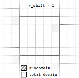Others: ¶

Parameter Name	FORTRAN Type	Default Value	Explanation
[=# ']
[=#<insert_parameter_name> <insert_parameter_name>]	<insert type>	<insert value>	<insert explanation>