Home

Context Navigation

Canopy model

The embedded plant canopy model allows for studying the turbulent flow inside and above vegetation canopy. It is well-known that vegetation canopy effects on the surface--atmosphere exchange of momentum, energy and mass can be rather complex and can significantly modify the structure of the ABL, particularly in its lower part (e.g., Raupach et al., 1996; Dupont and Brunet, 2009). It is thus not possible to describe such processes by means of the roughness length and surface fluxes of sensible and latent heat. The canopy model in PALM accounts for the vertically extended drag, release of heat, plant evaporation and leaf-air-interactions that are functions of height within the canopy layer.

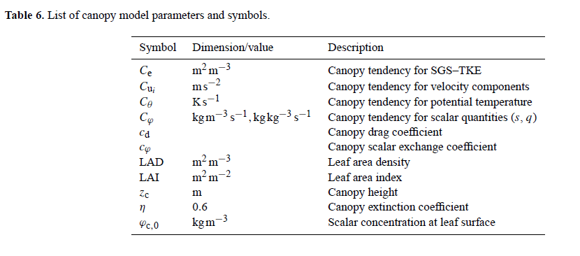
Dynamical effects of the plant canopy are based on the assumption that the canopy acts as a~sink for momentum due to form (pressure) and viscous drag forces. This sink for momentum is modeled following Shaw and Schumann (1992) and Watanabe (2004) by adding the term C_ui to the momentum equation (see Eq. one in Sect governing equations:

$\begin{align*} & \frac{\partial u_i}{\partial t} = \ldots - \underbrace{c_{\mathrm{d}}\,\text{LAD}\,\sqrt{u_i^2} u_{i}}_{C_{u_{i}}}\;. \end{align*}$

Here, C_ui represents the net resolved-scale dynamical effect of the canopy, averaged over the respective grid volume. c_d is the canopy drag coefficient with typical values around 0.2 (e.g., Cescatti and Marcolla, 2004), and LAD is the leaf area density (available leaf area per unit volume). As an example, LAD is rather constant with height within crop fields, whereas it is often very heterogeneous in forests, where most of the leaf area is concentrated in the trees' crown space (e.g., Yi, 2008).

The effect of the canopy on the SGS turbulence is considered by adding a similar sink term to the prognostic equation for SGS-TKE (see Sect. turbulence closure:

$\begin{align*} & \frac{\partial e}{\partial t} = \ldots - \underbrace{2 c_{\mathrm{d}} \text{LAD} \sqrt{u_i^2}\,e}_{C_e}\;. \end{align*}$

This approach was suggested by Shaw and Schumann (1992) and is based on the assumption that SGS-TKE is dissipated by the canopy due to the rapid dissipation of wake turbulence in the lee of plant elements. This rapid break-down of turbulence is also known as the spectral shortcut (e.g., Shaw and Patton, 2003). This type of canopy model has been successfully applied by various authors to study turbulent flows inside and above homogeneous as well as heterogeneous canopies such as forest edges (Cassiani et al., 2008; Finnigan et al., 2009; Dupont and Brunet, 2009, among others).

In case of incoming solar radiation the plant canopy acts as a source for heat. It is assumed that this warming of the foliage by solar radiation results in a warming of the surrounding air. This process is considered by adding a source term C_θ to the prognostic equation for θ (see Eq. three in Sect governing equations:

$\begin{align*} & \frac{\partial \theta_\mathrm{l}}{\partial t} = \ldots + \underbrace{\frac{\partial Q_{\theta}}{\partial z}}_{C_\theta}\;. \end{align*}$

In order to account for the fact that solar radiation can penetrate different layers of the canopy, based on the leaf area, an exponential decay function for the upward vertical kinematic heat flux Q_θ after Brown and Covey (1966)is used. Q_θ is derived at each height inside the canopy by means of the downward cumulative leaf area index (LAI):

$\begin{align*} & Q_{\theta}(z)=Q_{\theta}(z_\mathrm{c})\,\exp\left(-\eta\,\text{LAI}\right), \end{align*}$

with

$\begin{align*} \text{LAI} = \int_{z}^{z_\mathrm{c}}\;{\text{LAD}}\,\mathrm{d}z \end{align*}$

where Q_θ(z_c) is the prescribed heat flux at the top of the canopy layer z_c and η is the extinction coefficient set to 0.6. Additionally, contributions by sinks/sources for q and s are considered in the canopy model by adding additional terms C_φ to the scalar transport equations (see Eqs. four and five in Sect governing equations):

$\begin{align*} & \frac{\partial \varphi}{\partial t} = \ldots - \underbrace{c_\varphi {\text{LAD}} \sqrt{u_i^2} \left(\varphi-\varphi_{\mathrm{c},0}\right)}_{C_\varphi}\;, \end{align*}$

where φ ∈ {q, s} and c_φ is a user-defined scalar exchange coefficient. φ_c,0 and φ are the scalar concentrations at a leaf surface and in the surrounding air volume, respectively. This approach is based on the assumption that the scalar sink/source strength depends on the concentration gradient between the leaf surface and the surrounding air (e.g., Watanabe, 2004).

Recent applications

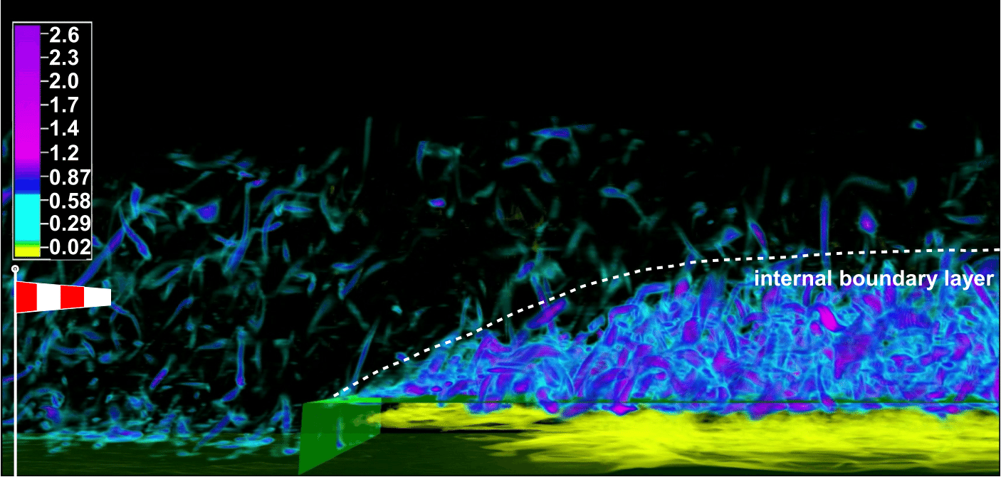
PALM simulations with the embedded canopy model were recently performed by Kanani et al. (2014c) to study the flow adjustment downstream of a transition from an unforested (clearing) to a forested surface patch. In this study the LES results were validated against multidimensional field and wind-tunnel data. In the high-resolution follow-up study of Kanani-Sühring and Raasch (2015), a detailed analysis of the turbulent scalar transport within the canopy layer was successfully performed for the first time by means of LES. Figure 11 shows exemplarily the flow at a forest edge, where an internal boundary layer developed above the forest due to the extended drag of the canopy. See also associated animations in Kanani et al. (2014a, b).

Figure 11: Snapshot of the absolute value of the 3-D rotation vector of the velocity field above a forest canopy downstream of a grassland-to-forest transition (forest volume marked by green isosurface). Pink and yellow colors illustrate strong and weak turbulence, respectively. A neutrally-stratified open-channel flow was simulated with the mean flow direction from left to right, i.e. perpendicular to the windward forest edge, using an equidistant grid spacing of 3 m. The figure shows only a subregion of the simulation domain (2 x 1 x 0.4 km³).

Plant canopies in complex terrain and urban environments

The detailed simulations of a complex environment e.g. of urban areas require modeling of the plant canopy (PC) in detail of the individual treetops. The PIDS allows to initialize model PALM-4U with arbitrary structure of the plant canopy leave area density (LAD) and basal area density (BAD). This allows to describe the complete 3D structure of individual trees and shrubs as well as the structure of tree clusters.

Integration of plant canopy and radiative transfer model (RTM)

While the dynamical effects of such complex vegetation structure can be treated in the way described above, the interaction with radiation requires a deep integration with RTM. This integration is described in detail in RTM documentation. The direct, diffuse, and reflected short wave and lond wave radiation is partialy absorbed by individual grid boxes of PC and transformed to sensible heat flux inside the vegetation. This heat flux is consequently transformed to increase of the corresponding air mass. The PC also emmits the long wave radiation according its current local temperature.

Calculation of plant canopy latent heat fluxes

An important part of the heat balance in the urban canopy represent the latent heat fluxes from the vegetation. The RTM explicitly computes the radiation balance for each grid cell of the volumetric plant canopy which allows to calculate the evapotranspiration of this vegetation.

The evapotranspiration of the resolved vegetation is modelled using the Jarvis-Stewart method (Stewart, 1988) implemented following Daudet et al. (1999) as

$\begin{align*} & E = \Omega E_\mathrm{eq} + (1 - \Omega) E_\mathrm{imp} , \end{align*}$

where E_eq is the equilibrium evaporation per leaf unit area, E_imp the imposed evaporation per leaf unit area and Ω is the decoupling factor. These variables are modeled as

$\begin{align*} & l_\mathrm{v} L_\mathrm{eq} = \frac{R_\mathrm{n}\frac{q_\mathrm{s}}{\gamma}}{\frac{q_\mathrm{s}}{\gamma}+2}, \\ & l_\mathrm{v} E_\mathrm{imp} = {\rho} c_p g_\mathrm{s} e_{p,d} {\gamma}, \\ & \Omega = \frac{\frac{q_\mathrm{s}}{\gamma}+2}{\frac{q_\mathrm{s}}{\gamma}+2+ 2g_\mathrm{b} /g_\mathrm{s}}, \end{align*}$

where R_n is the net radiation calculated by the RTM for each grid cell containing vegetation, e_d = e_s − e is the water vapor pressure deficit in the air (with e_s and e being the water vapor pressure at saturation and the water vapor pressure, respectively), q_s = ∂e_s /∂T is the partial derivative of the water vapor saturation pressure with respect to temperature, γ = (c_p p)/(0.622 l_v) is the psychrometric constant, g_b is the leaf boundary layer conductance and g_s is the stomatal conductance. The leaf boundary layer conductance is parametrized as (Daudet et al., 1999)

$\begin{align*} & g_\mathrm{b} = 0.01{\text{U}} + [0.0071]\mathrm{ms}^{-1}. \end{align*}$

The stomatal conductance is parameterized after Stewart (1988):
$\begin{align*} & g_\mathrm{s} = g_\mathrm{s,max} f_1(SW_\downarrow) f_2(T) f_3(e_d) f_4(RSWC), \end{align*}$

where g_s,max is the maximum value of the stomatal conductance and f₁–f₄ dimensionless empirical functions that express the dependence of the conductance on the incoming shortwave radiation SW↓, air temperature T , water pressure deficit e_d and the relative soil water content RSWC.

After computing the evaporation per unit leaf area E, the latent heat flux from leaves per the unit volume of vegetation is calculated by multiplication by the leaf area density LAD

$\begin{align*} & LE = l_\mathrm{v} \,{E}\, \text{LAD} \end{align*}$

and the sensible heat flux is the residual of the energy balance, neglecting the storage.

References

Daudet, F. A., et al. 1999. Wind speed and leaf boundary layer conductance variation within tree crown: consequences on leaf-to-atmosphere coupling and tree functions. Agricultural and Forest Meteorology 97.3: 171-185.

Stewart, J. B. 1988. Modelling surface conductance of pine forest. Agricultural and Forest meteorology 43.1: 19-35.

Raupach MR, Finnigan JJ, Brunet Y. 1996. Coherent eddies and turbulence in vegetation canopies: the mixing-layer analogy. Bound.-Lay. Meteorol. 78: 351–382.

Dupont S, Brunet Y. 2009. Coherent structures in canopy edge flow: a large-eddy simulation study. J. Fluid Mech. 630: 93–128.

Shaw RH, Schumann U. 1992. Large-eddy simulation of turbulent flow above and within a forest. Bound.-Lay. Meteorol. 61: 47–64.

Watanabe T. 2004. Large-eddy simulation of coherent turbulence structures associated with scalar ramps over plant canopies. Bound.-Lay. Meteorol. 112: 207–341.

Cescatti A, Marcolla B. 2004. Drag coefficient and turbulence intensity in conifer canopies. Agr. Forest Meteorol. 121: 197–206.

Yi C. 2008. Momentum transfer within canopies. J. Appl. Meteorol. 47: 262–275.

Shaw RH, Patton EG. 2003. Canopy element influences on resolved- and subgrid-scale energy within a large-eddy simulation. Agr. Forest Meteorol. 115: 5–17.

Cassiani M, Katul GG, Albertson JD. 2008. The effects of canopy leaf area index on airflow across forest edges: large-eddy simulation and analytical results. Bound.-Lay. Meteorol. 126: 433–460.

Finnigan JJ, Shaw RH, Patton EG. 2009. Turbulence structure above a vegetation canopy. J. Fluid Mech. 637: 387–424.

Brown KW, Covey W. 1966. The energy-budget evaluation of the micro-meteorological transfer process within a cornfield. Agr. Meteorol. 3: 73–96.

Kanani F, Träumner K, Ruck B, Raasch S. 2014c. What determines the differences found in forest edge flow between physical models and atmospheric measurements? -- an LES study. Meteorol. Z. 23: 33–49.

Kanani-Sühring F, Raasch S. 2015. Spatial variability of scalar concentrations and fluxes downstream of a clearing-to-forest transition: a large-eddy simulation study. Bound.-Lay. Meteorol. 155: 1–27. doi.

Kanani F, Maronga B, Knoop H, Raasch S. 2014a. Large-eddy simulation of a forest-edge flow -- adjustment of a turbulent flow to the changing surface conditions at a clearing-to-forest transition. Computer animation. doi.

Kanani F, Maronga B, Knoop H, Raasch S. 2014b. Large-eddy simulation of the scalar transport in a forest-edge flow -- spatial variability of the scalar distribution and the scalar transport downstream of a clearing-to-forest transition. Computer animation. doi.

Last modified 5 years ago Last modified on Oct 1, 2019 6:24:47 AM

Attachments (2)

09.png (334.6 KB) - added by kanani 7 years ago.
Table6.png (32.0 KB) - added by schwenkel 6 years ago.

Download all attachments as: .zip

Download in other formats:

Plain Text